International Journal of Computer Science and Engineering Volume 1 Number 2
Image Magnification Using Adaptive Interpolation by Pixel Level Data-Dependent Geometrical Shapes Muhammad Sajjad, Naveed Khattak, and Noman Jafri magnify the original images. Therefore, the development of a good image magnification algorithm is very important. Until now, a large number of interpolation techniques for magnifying images have been proposed. A typical problem with most interpolation techniques is that although smoothing the data and keeping the low frequencies in the new zoomed picture, they are not able to enhance the high frequencies or preserve the edges equally well. Visually those problems will result in either blurring or blocking artifacts. A possible solution would need a sort of non-linear interpolation, taking into account the directional variation for maintaining the sharpness of the new enlarged image and smoothness as well. The simplest method to magnify images is the pixel replication. However, the resulting magnified images have aliasing effect in the form of jagged edges. Nearest neighbor interpolation is the simplest method and basically makes the pixels bigger. The color of a pixel in the new image is the color of the nearest pixel of the original image[4]. Most image viewing and editing software use this type of interpolation to enlarge a digital image for the purpose of closer examination because it does not change the color information of the image and does not introduce any anti-aliasing. For the same reason, it is not suitable to enlarge photographic images because it increases the visibility of jaggies. More elaborate approaches use the bilinear or the bicubic interpolation. Bilinear Interpolation determines the value of a new pixel based on a weighted average of the 4 pixels in the nearest 2 x 2 neighborhood of the pixel in the original image [4]. The averaging has an anti-aliasing effect and therefore produces relatively smooth edges with hardly any jaggies. Bicubic interpolation is more sophisticated and produces smoother edges than bilinear interpolation. Here, a new pixel is a bicubic function using 16 pixels in the nearest 4 x 4 neighborhood of the pixel in the original image [1, 4]. This is the method most commonly used by image editing software, printer drivers and many digital cameras for resampling images. Commercial software Adobe Photoshop [1] provides these two functions for interpolating images. Other methods, using the B-spline interpolators [8, 11] or the cubic convolution methods [10] have also been proposed. However, these methods tend to blur the edges and cause them to be jagged. Research on interpolating images taking into account the edges, has gained much attention. Allebach and Wong [2] proposed methods that search for edges in the input image and use them to assure that the interpolation does not cross
Abstract—World has entered in 21st century. The technology of computer graphics and digital cameras is prevalent. High resolution display and printer are available. Therefore high resolution images are needed in order to produce high quality display images and high quality prints. However, since high resolution images are not usually provided, there is a need to magnify the original images. One common difficulty in the previous magnification techniques is that of preserving details, i.e. edges and at the same time smoothing the data for not introducing the spurious artefacts. A definitive solution to this is still an open issue. In this paper an image magnification using adaptive interpolation by pixel level data-dependent geometrical shapes is proposed that tries to take into account information about the edges (sharp luminance variations) and smoothness of the image. It calculate threshold, classify interpolation region in the form of geometrical shapes and then assign suitable values inside interpolation region to the undefined pixels while preserving the sharp luminance variations and smoothness at the same time. The results of proposed technique has been compared qualitatively and quantitatively with five other techniques. In which the qualitative results show that the proposed method beats completely the Nearest Neighbouring (NN), bilinear(BL) and bicubic(BC) interpolation. The quantitative results are competitive and consistent with NN, BL, BC and others.
Keywords—Adaptive, digital image processing, image magnification, interpolation, geometrical shapes, qualitative & quantitative analysis.
T
I. INTRODUCTION
ODAY, there is a huge amount of digital images available to computer users. This is caused by the rapid growth both in computer hardware and software technologies. Low price digital cameras are now common, and as a result users are able to buy them and take as many digital images as desired. The significant development in the field of computer graphics has also boosted the production of digital images. As computer users become more familiar with digital images, the need to display and print them also increases. In an era where highresolution display and printing devices are common, it is vital that high-resolution images are available in order to produce high quality displayed images and high quality prints. This is particularly important for desktop publishing, large artistic printing, etc. The problem is that high-resolution images are not usually provided. In these cases, there is a need to Authors are with Department of computer Science, College of signals, National University of Sciences and Technology, Rawalpindi, Pakistan (email:
[email protected], {khattakn, mnjafri}@mcs.edu.pk).
118
International Journal of Computer Science and Engineering Volume 1 Number 2
proposed technique is so intelligent that it can differentiate between low and high frequency content of the source image and thus it preserve the visual sharpness of the original image. The proposed technique is very easy to implement and efficient as well than other proposed techniques. The quantitative and qualitative analysis of proposed technique shows that it has covered some of the weakness of other proposed technique up to some extent with respect to quality and efficiency.
them. The problem is one of how to define and find the important edges in the input image. Other edge-adaptive methods have been proposed by Jensen and Anastassiou [9], Li and Orchard [12], and Muresan and Parks [15, 16, 17, 18] . Currently, the methods presented in [12, 18] are the most widely known edge-adaptive methods. They can well enough avoid jagged edges, but a limitation is that they sometimes introduce highly visible artifacts into the magnified images, especially in areas with small size repetitive patterns. X. Yu, B. Morse, T.W Sederberg [19] presented a method that computes a triangulation of the input image where the pixels in the input image are the vertices of the triangles in the triangulation. The input image at any arbitrary scale is reconstructed by rendering its triangulation. However, since the edges in the input image are approximated using piecewise linear segments, curved edges cannot be properly reconstructed especially when the scaling factor is a large number. Morse and Schwartzwald [14] presented a level-set reconstruction method to solve the problem of jagged edges. Their approach starts by magnifying the input image using the bicubic interpolation method, then iteratively smoothing the contours in the image. This approach, however, does not overcome the blurring problem found in the bicubic interpolation method. Hertzmann et al. [7] and Freeman et al. [3] proposed methods that learn the correspondences between low and high resolution images from a set of training data. The advantage of these approaches is that fine details can be added when producing high-resolution images when the input image is in the same class of image as the training data. The disadvantages of these approaches are that they will fail if the input image is not in the same class as the training data and that the computational cost is high. Variational based approaches for image magnification have been presented by Malgouyres and Guichard [13]. The magnified images obtained using these methods are better than those obtained using the bicubic interpolation method. However, since these methods solve optimization problems where all the pixels in the magnified image are unknowns, these methods, too, have high computational costs. As a result, they are not suitable for practical use. Another good approach is presented by Henry Johan and Tomoyuki Nishita [5] which produces a high quality magnified image. They have proposed a progressive refinement approach for image magnification. They also claimed for sharp magnified image without generating distinct artifacts but some times it also produce jaggeis to magnify the image. Muneeb, Naveed khattak (KM) [6] and . Battiato, G. Gallo, and F. Stanco[20] also proposed an adaptive approach for image magnification which produces a high quality magnified image while preserving information contents of original image but it has also some defects. These [6, 20] has also been considered in qualitative and quantitative analysis of this paper. The main contribution of this paper is to produce an enlarge image with high visual quality of the original image. The basic idea of the proposed technique is to separate the interpolation region in the form of geometrical shape and then the interpolator assign a proper intensity value to the undefined pixel inside this interpolation region. It does not require a preliminary gradient computation because the relevant information is collected during magnification process. The
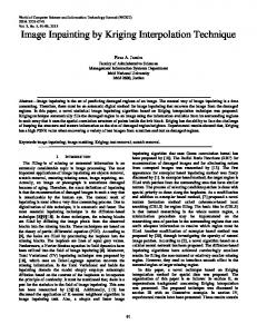
II. THRESHOLDING Because of its intuitive properties and simplicity of implementation, image thresholding play a vital roll in application of digital image processing. In image magnification thresholding also plays a key roll in preservation of edges. So it’s most important to select a suitable threshold during interpolation to preserve the fine detail of the image. To preserve the visual quality of the image, the threshold on the basis of safe color [21] is calculated. There are 16 true gray shades from 0 to 255 which can be differentiated visually.
Fig. 1 Sixteen Safe Gray Colors in the 256-Color RGB System
As in Fig. 1 there are 16 safe colors out of 256. If ‘256’ is divided by ‘16’ we will get 16 as a Quotient. It means that after adding 16 to any gray shad then it will change its visual depiction. To calculate the threshold ‘T‘ for the preservation of the edge using above concept. If N is equal to 16 and where X1=0, X2=2 ,.......... XN=15 and Median denoted by Md is defined as: Md = (XN/2 + XN/2+1) /2
(1)
T= Md
(2)
It has been proved experimentally that it gives excellent result in preservation of edges during magnification and this threshold is also considered during magnification process. III. CLASSIFICATION OF INTERPOLATION REGIONS AND GEOMETRICAL SHAPES Edge preservation plays very important roll in magnification because it specifies the interpolation region in which interpolator adopt itself according to the region. To consider all possible interpolation region during magnification algorithm and assign a suitable value to the undefined pixel is very important. The concept relies on using the low resolution(LR) image to find zero crossing that indicate the presence of an edge passing through LR unit cell. These zerocrossing are then linked by straight line segments to obtain an estimate of the edge which divide the region in different interpolation region. The zero crossing are determined by applying Second order derivative on the LR image then for every LR unit cell after applying 2nd derivative the absolute value either on each side of the zero is compared to the threshold calculated in section 2. If the value is greater than
119
International Journal of Computer Science and Engineering Volume 1 Number 2
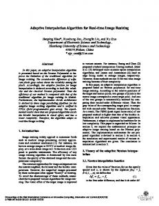
threshold it mean that the point of high contrast is present as shown in Fig. 2.
Fig. 4 3 D visualization of Fig. 3
As in Fig. 4 all the pixels are at the same level and it create a shape of square which consist only on one interpolation region. B. LR Region with Corner Edges The LR unit cell where an edge separates one pixel from the other three pixels of the LR unit cell. When the point of high contrast separate one pixel from the other three i.e. this pixel will have a value substantially different to the other three. This also call the outlier, imagine in Fig. 5.
Fig. 2 Determination of zero-crossing and its parameter
In Fig. 2 sequence of LR samples from some function f are given. Now calculate the point of high contrast by applying ∂2f /∂2x on sequence of LR unit cell of some function f. After calculation the magnitude on either side of zero-crossing is compared as in equation 3. ∂2f /∂2x = f (xLR2) + f (xLR0) - 2f (xLR1) │∂2f /∂2x │ > T
(3)
If the above statement is true then it mean that there is point of high contrast i.e. edge is present. So to make the above description as a base, a LR (original image) unit cell is analyzed consist on four pixels and determines the point of high contrast to categorize the edges, which split the LR unit cell into different interpolation and its orientation. In this way the interpolation regions are classified which make different geometrical shapes.
Fig. 5 LR unit cell where edge separate one corner from the other three i.e. two interpolation regions
In Fig. 5 color difference of pixels show intensity difference which has been explained above. This intensity difference split the LR unit cell in two interpolation region. It has been visualized in the following Fig. 6.
A. Constant Region The LR unit cell which has not any point of high contrast among the pixels is a linear area. It consists only on one interpolation region.
Fig. 6 Triangulation in a four-pixel square
In Fig. 6, pixels with same intensity level form a shape of triangle. This triangle has been considered one interpolation region. There are four possible cases of triangulation, which form triangle in different direction. So there are four different cases in which one pixel isolate from other three and in this way it divide the LR unit cell into two interpolation regions. The remaining cases have been shown in the next Fig. 7.
Fig. 3 Area where no edge passing through an LR unit cell In Fig. 3 circles show pixels and their color content shows intensity level. All the pixels are at the same level of intensity, so the resultant region is linear and the total number of interpolation region is one, it has also been visualize in the form three dimensions as in Fig. 4.
120
International Journal of Computer Science and Engineering Volume 1 Number 2
Now all the information is at hand about the interpolation regions. This information will be used in the implantation of algorithm. Due to this basic information the result of proposed algorithm has improved qualitatively and quantitatively as well. The concept of this section will be used in the coming section ‘The Basic Concept of Algorithm’. IV. THE BASIC CONCEPT OF ALGORITHM In this section the detail description of the basic concept of proposed algorithm is described. First the proposed algorithm is explained for gray scale images and then it is generalized for colour images. Algorithm works in four phases. This has been described in this section. In the first phase of the proposed algorithm the input image is expanded. Suppose the size of the input image is n x m where ‘n’ is number of rows and m is the number of columns. The image will be expanded to size of (2n-1) x (2m-1). The question arises that why one is subtracted from rows and columns. If it is not subtracted then there will be one additional row and column of undefined pixels which will have the intensity value of the adjacent row and column respectively. This is a sort of replication and the replication has been avoided completely in proposed algorithm.
Fig. 7 Triangulations in a four-pixel square
In Fig. 7 these triangle in different direction are considered different interpolation region. If one pixel isolate itself form other pixels due to intensity difference in all scenarios, whatever the intensity difference, all three pixels will be considered in same region of triangle which has been shown above. C. LR Region with Horizontal and Vertical Edeges In this scenario edge separate a pair of pixels from other pair of pixels i.e. it split the LR cell in two horizontal or vertical regions having contrast intensity.
Fig. 8 Edge which split the LR unite cell vertically
Fig. 11 Expansion phase showing source image (n x m) and expanded image (2n-1) x (2m-1)
In Fig. 9, one pair of pixels is on same side having different intensity level from other pair of pixels is on opposite side. So in such type of scenarios LR unit cell will be split horizontally or vertically.
In Fig. 11, solid circles show original pixels and hollow circles show undefined pixels. In the remaining three phases these undefined pixels will be filled with proper intensity values while preserving details and edges of original image and data smoothing. The second phase of the algorithm is most important one. In this phase the interpolator assign value to the undefined pixel by pixel level data dependent geometrical shapes.
Fig. 9 Square split by edge into two interpolation region
The same process can be repeated for the horizontal case. Here important is the splitting of two poles, whether it is vertically or horizontally. If the intensity contrast occurs horizontally the shape of the LR unit cell will be become as in Fig. 10.
Fig. 12 HR unit cell with undefined pixels Top, Center, Bottom, Left, Right denoted by T, B, C, L, R respectively
As it has been mentioned that the assignment of proper intensity value to the undefined pixel is depend on the pixel level data dependent geometrical shapes. In this phase the algorithm scan the image and each time it consider the group of pixels as shown in Fig. 12 and checks that what type of
Fig. 10 Edge which split the LR unit cell into two horizontal interpolation regions
121
International Journal of Computer Science and Engineering Volume 1 Number 2
geometrical shape form here. After confirmation of geometrical shape, it assigns value to the undefined pixel. If the region is constant and there is no point of high contrast among the defined pixels of the High resolution (HR) cell as shown in Fig. 12. It will be confirmed by calculating the standard deviation of defined pixels in HR cell. σ=
(X − Xi )2 + (X − Xi − 1)2 + (X − Xi − 2)2 + (X − Xi − 3)2 N
2*σ