3112
IEEE TRANSACTIONS ON IMAGE PROCESSING, VOL. 20, NO. 11, NOVEMBER 2011
Image Magnification Using Interval Information Aranzazu Jurio, Miguel Pagola, Radko Mesiar, Gleb Beliakov, Senior Member, IEEE, and Humberto Bustince, Member, IEEE
Abstract—In this paper, a simple and effective image-magnification algorithm based on intervals is proposed. A low-resolution image is magnified to form a high-resolution image using a block-expanding method. Our proposed method associates each pixel with an interval obtained by a weighted aggregation of the pixels in its neighborhood. From the interval and with a linear operator, we obtain the magnified image. Experimental results show that our algorithm provides a magnified image with better quality (peak signal-to-noise ratio) than several existing methods. Index Terms—Image magnification, implication operator, interval, operator.
I. INTRODUCTION
I
MAGE-MAGNIFICATION methods attempt to increase the spatial resolution of an image without introducing a blur. This process is also known as superresolution [1], [2], image scaling [3], upsampling [4], zooming [5], and image enlargement [6] in related literature. Image magnification is currently a very active area of research as it is used in many applications. For instance, it can overcome resolution limitations of low-cost imaging systems of personal digital assistants, mobile phones, or surveillance cameras. It is also considered as key medical- and satellite-imaging techniques where the diagnosis or analysis in enhanced resolution images is desired. Additionally, there exists a great demand of video sequence enhancement [7] due to the fact that most web videos are limited by network bandwidth and server storage; thus, it should be stored in low quality. Previous works on image magnification can be roughly divided into three categories: 1) reconstruction methods; 2) approaches based on machine learning techniques; and 3) interpolation methods. Manuscript received August 24, 2010; revised January 26, 2011 and April 06, 2011; accepted May 16, 2011. Date of publication May 31, 2011; date of current version October 19, 2011. This paper was supported in part by the National Science Foundation of Spain under Grant TIN2010-15055, by the Research Services of the Universidad Publica de Navarra, by Grant VEGA 1/0080/10, and by Grant P402/11/0378. The Associate Editor coordinating the review of this manuscript and approving it for publication was Prof. A. A. Ross. A. Jurio, M. Pagola, and H. Bustince are with the Departamento de Automatica y Computacion, Universidad Publica de Navarra, 31006 Pamplona, Spain (e-mail
[email protected];
[email protected];
[email protected]). R. Mesiar is with the Department of Mathematics and Descriptive Geometry, Slovak University of Technology, 813 68 Bratislava, Slovakia, with the Institute of Information Theory and Automation, Academy of Sciences of the Czech Republic, 18208 Prague, Czech Republic, and also with the Institute for Research and Application of Fuzzy Modeling, University of Ostrava, 70103 Ostrava, Czech Republic (e-mail:
[email protected]). G. Beliakov is with the School Information Technology, Deakin University, Burwood 3125, Australia (e-mail:
[email protected]). Digital Object Identifier 10.1109/TIP.2011.2158227
The reconstruction task is based on prior knowledge about the model that maps the high-resolution image to the low-resolution one. The magnification is then considered as the inverse problem: recovering the original high-resolution image by fusing one or more low-resolution images [8]. In the approaches based on machine learning methods [9]–[11], a set of examples of low resolution and their ideal high-resolution patches are organized in a database. The main idea consists on seeking in the database for similar low-resolution examples, given a patch from the low-resolution input. Their corresponding high-resolution counterparts can then be used for the reconstruction. The most frequently used methods working with a single image are based on interpolation [12]. Common algorithms, such as nearest neighbor or bilinear interpolation, are computationally simple but suffer from smudge problems, particularly in the edge areas. Directional image interpolations take advantage of the geometric regularity of image structures by performing the interpolation in a chosen direction along which the image is locally regular. Therefore, many adaptive interpolations have been developed with edge detectors [4]. Nevertheless, linear approximations are the most used ones since their computational cost is lower. Our goal in this paper is to develop a cost-efficient method to construct, starting from a given image, a new image of larger size such that each area or block in the new image is obtained by a weighted aggregation of the intensities of the pixels in the neighborhood of each pixel in the original image. To reach this goal, the method that we propose makes use of the notions of operators [13]. We use intervals because it has interval and been proven in image processing that they allow keeping information about the neighborhood of each pixel [14]. In this way, we employ that information to get the intensities of the new operators bepixels in the magnified image. We also use cause they allow us to choose, depending on the parameter, the internal point of the interval that we must select. To associate an interval to each pixel within the image, we present a new construction method of intervals from a pixel and its neighborhood. We are going to understand the length of this interval as a measure of the variation of intensities in the neighborhood of each pixel. To see that our method is computationally simple and gets good results, we compare the images obtained by our algorithm and the ones obtained by other methods, both classical and more recent ones. This paper is organized as follows: First, in Section II, we recall some preliminary definitions. In Section III, we show the method to construct intervals. In Section IV, we present the image-magnification algorithm. We finish with some experimental results in Section V and conclusions in Section VI.
1057-7149/$26.00 © 2011 IEEE
JURIO et al.: IMAGE MAGNIFICATION USING INTERVAL INFORMATION
II. PRELIMINARIES In this section, we recall the main concepts that are necessary for subsequent developments. A strictly decreasing and continuous function , such that and , is called strict negation. If, in addition, is involutive , then we say that it is a strong negation. We call automorphism of the unit interval every function that is continuous, strictly increasing, and such that and . Let us denote by the set of all closed subintervals in [0, 1], that is and is a lattice with respect to the relation defined in the following way, given , if and only if
, which is , we have
and
From now on, we denote by the length (width) of the considered interval; that is, . Definition 1: Let . The operator is given by
for all . Clearly, the following properties hold. a) for all . b) for all . c) for all . Notice that operator is a particular case of the Hurwicz aggregation function [15].
3113
this section, we propose a construction method of the elements of from two points in [0, 1], such that the first number is an internal point of the interval and the second number represents the length of the interval. The construction method is described in the following theorem. Theorem 1: Let be such that (F1) for all ; (F2) is increasing in the first variable; (F3) is decreasing in the second variable; (F4) for all . Then, , , for all , and mapping given by
is such that for all , . Proof: By construction, . From (F4), for all . By (F2), . Thus, is well defined. Due to (F1) and (F3), . by construction. From (F2), by (F4). As and , by (F3). In the following lemma, we relate our operator that generates intervals with implication operators. This result is really useful because implication operators have been widely studied; thus, we can use several expressions of implication operators to create functions. Lemma 1: Let be such that (F1)–(F4) hold. Then, mapping given by
A. Implication Operators Definition 2:
An implication operator is function that satisfies the following properties
[16]. : implies for all . : implies for all . : for all (dominance of falsity). : for all . : . Remark: Properties , , and imply that is an extension of the standard Boolean implication operators. Indeed, it holds , and . We follow the notation presented in [16], where other properties can be found. In particular, we will use the following ones throughout this paper. : (neutrality of truth). : (exchange property). : where is a strong negation. : is a continuous function (continuity). III. CONSTRUCTION OF INTERVALS OF FIXED LENGTH In our algorithm, we represent the information of the neighborhood of each pixel by an interval. We use this interval to construct the intensities of the new pixels in the magnified image. In
is an implication operator for any strict negation . Proof: and follow from (F2) and (F3). . . from (F4). In the following theorem, we present a characterization of the construction method. Theorem 2: Mapping satisfies properties (F1)–(F4) if and only if there exists an implication operator satisfying with respect to the standard negation and such that
Proof: (Sufficiency) is decreasing in the first variable and increasing in the second, from (F2) and (F3). . . ; thus, . . (Necessity) from . (F2) and (F3) from the monotonicity properties of . from . Example 1: In this example, we present some expressions of functions constructed from different implication operators. a) Consider Kleene–Dienes implication and standard negation. Then,
3114
IEEE TRANSACTIONS ON IMAGE PROCESSING, VOL. 20, NO. 11, NOVEMBER 2011
. In this way, the resulting interval is (1) and .
b) Take Reichenbach implication standard negation. Then, Thus, the resulting interval is
(2) c) Take Lukasiewicz implication dard negation. Then, . Thus, the resulting interval is
Fig. 1. How to select grid . For the magnification of the pixel in dark gray, all the pixels in (dark and light) gray belong to grid . (a) The case where the magnification factor is (2 2). (b) The case where the magnification factor is greater than or equal to (3 3).
and stan-
(3) Remark: From now on, we will use the standard negation as . The following theorem is the basis for the image-magnification algorithmic construction that we present in Section IV. It is used to keep the intensity of each pixel from the original image in the new magnified image. Theorem 3: In the setting of Theorem 2, the following item holds: if and only if (Reichenbach's implication). Proof: (Necessity) Thus,
. . (Sufficiency) . Theorem 4: If with for all , , then for all . Proof: If , then . , and . In the next corollary, we build mappings from automorphisms. Corollary 1: Let be such that (F1)–(F4) hold. Suppose that the implication operator given by Theorem 2 satisfies , , and . In these conditions, there exists an automorphism in the unit interval such that (4) Proof: Direct from the result, proved in [16]. Remark: Notice that for (4) to satisfy take . Therefore, Example 2: If we take , then (Reichenbach’s implication).
, it is necessary to .
IV. MAGNIFICATION ALGORITHM We consider image as an matrix. Each coordinate of the pixels in image is denoted by . The normalized intensity or normalized gray level of the pixel located at is represented as , with for each .
Fig. 2. How to select grid for different magnification factors: (a) factor (2 2), (b) factor (3 3), (c) factor (4 4), and (d) factor .
The purpose of our algorithm is, given image of dimension , to magnify it times; that is, to build a new image of dimension with , , and , with and . We denote as a magnification factor. To do so, we use two different grids over each pixel in the original image, in the following way: 1) Grid from which we will calculate an interval of intensities. This block captures the variability of the intensities in the pixel’s neighborhood. The size of this window is with , , such that and . The values of and depend on the magnification factor (see Fig. 1). 2) Grid whose size is (see Fig. 2). We use this grid and the interval calculated before to build a new block of size in the magnified image. The scheme of our algorithm is illustrated in Fig. 3. The image on the left is the original one. We assign to the pixel the expanded block of the same size as (in this example, ; hence, is a 3 3 block). The image on the right corresponds to the result of the algorithm. Algorithm 1 presents the method we propose using grids , , and . In it, we can see that this method is characterized by its simplicity from the implementation point of view.
JURIO et al.: IMAGE MAGNIFICATION USING INTERVAL INFORMATION
3115
Fig. 4. Example: Original image.
Fig. 3. Magnified image with
.
Algorithm 1 INPUT:
original image,
magnification factor.
1. Select ,
.
2. FOR each pixel
DO
2.1 Fix a grid
of dimension
Fig. 5. Example: Original image.
centered at
.
2.2 Calculate as the difference between the largest and the smallest intensities of the pixels in . , where 2.3 Calculate the standard deviation of the intensities of using (2).
2.4 Build the interval 2.5 Fix a grid
, being .
of dimension
of size
2.6 Build a new empty block 2.7 FOR each element
centered at
of
.
.
DO
ENDFOR 2.8 Put the block
in the magnified image.
which is analogous for and . We just use the set of values because the greater the size of the grid , the greater the neighborhood of each pixel that we consider, and we do not want that remote pixels interfere in the magnification. In the example, we want to magnify the image by factor (3 3); therefore, . B. Step 2.1: Fix Grid Pixel
of Dimension
Centered at Each
This grid represents the neighborhood that is used to build the interval. In the example, for pixel (2, 3) (marked in dark gray in Fig. 5), we fix a grid of dimension around it (in light gray). Remark: For pixels in the first or the last row/column, we choose a grid centered at them, as shown in Fig. 6. C. Step 2.2: Calculate as the Difference Between the Largest and the Smallest of the Intensities of the Pixels in is the maximum length that the interval we are going to build can have, i.e.,
ENDFOR Next, we explain the steps of Algorithm 1 by means of an example. Given an image in Fig. 4 of dimension 5 5, we want to build a magnified image of dimension 15 15 magnification factor .
(5) In the example, for pixel (2, 3), we calculate
as
A. Step 1: Select , These parameters represent the size of grid . Their values ( for rows and for columns) are selected depending on the following magnification factor: if else if else
then then
D. Step 2.3: Calculate represents the length of the interval that we build. Our first idea was to use as the length of the interval (instead of ) in our construction. However, that proposal has some
3116
IEEE TRANSACTIONS ON IMAGE PROCESSING, VOL. 20, NO. 11, NOVEMBER 2011
Fig. 6. Example: Grid for pixels in the first or last row/column. (a) Pixel in the first column. (b) Pixel in the last column. (c) Pixel in the first row. (d) Pixel in the last row. Fig. 8. Solution to the problem in Fig. 7 using
Fig. 9. Original
parameter.
block for pixel (2, 3).
Following the example in Fig. 4, the standard deviation of grid is 0.0834; thus, . Then, the length for the interval associated to pixel (2, 3) is . E. Step 2.4: Build Interval Fig. 7. Problem with the edges in binary images if the amplitude is
.
problems, as it is shown in the example in Fig. 7. In the upper part, it is the numerical calculation and below is its representation in the image, where 0 means black and 1 means white. As we can see, the edge in the magnified image is not correct. To solve this problem, the length of the interval is proportionally reduced to parameter , and in this way, the jump from white to black is gradual. To calculate the value, we use the standard deviation of the intensities in grid . We use the expression because the maximum standard deviation in grid is 0.5, and we want the value to vary in [0, 1]. In this sense, if all the pixels in have the same intensity, the amplitude of the interval is ; nevertheless, when there is a big difference between the intensities (presence of an edge), the value of decreases, and therefore, the amplitude also decreases. Fig. 8 shows the effect of parameter .
We associate to each pixel an interval of length . To do so, we use the method explained in Section III. In this case, we take the expression in (2) based on Reichenbach’s implication. The resulting interval is
In the example, the interval associated to pixel (2, 3) is given by
F. Step 2.5: Fix Grid
of Dimension
Centered at
In the example, this new block is shown in Fig. 9. G. Step 2.6: Build a New Empty Block
of Size
Following the example, the size of this block is 3 Fig. 10).
3 (see
JURIO et al.: IMAGE MAGNIFICATION USING INTERVAL INFORMATION
Fig. 10. Empty block
3117
.
Fig. 13. Schema to check the algorithm.
Fig. 11. Expanded block for pixel
.
Fig. 14. Images used in the different factors experiment. (From left to right) Ship, Lena, and Peppers.
TABLE I PSNRS (IN DECIBELS) OVER IMAGES IN FIG. 14. (FROM LEFT RIGHT) IMAGES MAGNIFIED BY FACTORS (1 2), (2 1), (2 2), (3 3), AND (4 4)
Fig. 12. Numerical expanded block for pixel
H. Step 2.7: Calculate
TO
.
for Each Pixel
Next, we expand pixel in image over the new block . In the example, pixel (2, 3) is expanded, as shown in Fig. 11. To keep the value of the original pixel at the center of the new block, Theorem 3 states that should be equal to the intensity of that pixel. In the case of pixel (2, 3), we have
We apply this method to fill in all the other pixels in the block. In this way, from Proposition 3, we take as for each pixel the value of that pixel in the grid . • . Then, . • . Then, . • • . Then, . In Fig. 12, we show the expanded block for pixel (2, 3) in the example. Once each of the pixels has been expanded, we join all the blocks (Step 2.8) to create the magnified image. This process is shown in Fig. 3. V. EXPERIMENTAL RESULTS To quantitatively estimate the quality of magnification, we take a set of gray-scale images of size 512 512 and reduce
them to several sizes (see Section V-A). Then, we enlarge the previously reduced images back to 512 512 and compare them to the images from which we started. Our expectation is that the enlarged images will be similar to the original ones, and we can estimate the similarity quantitatively by the peak signal-to-noise ratio (PSNR). In Fig. 13, we see a schema of the procedure when we reduce the image to obtain a 9 smaller one and then enlarge the result by the magnification factor (3 3). A. Reduction Algorithm To reduce the images, we use the algorithm proposed in [17]. , the scheme of Starting from the images of dimension the algorithm is the following. 1) Divide image in blocks of size . If is not a multiple of or of , we delete the minimum number of rows/ columns in the boundary of the image until the new size of the image satisfies the property. 2) Associate each block with an interval in the following way: The lower bound of the interval is given by the minimum of the intensities in the block and the upper bound, by the maximum. 3) Associate each interval with the middle point of the interval. We select this reduction algorithm because it takes into account all the pixels of the block, instead of other reduction methods such as subsampling (take one of every pixels).
3118
IEEE TRANSACTIONS ON IMAGE PROCESSING, VOL. 20, NO. 11, NOVEMBER 2011
Fig. 15. (a) Reduced image Ship of size 256 256 and its magnification by (b) factor (1 2) of size 256 512, (c) factor (2 1) of size 512 256, and . (e) Reduced image Ship of size 170 170 and (f) its magnification by factor (3 3) of size 510 510. (g) Reduced image (d) factor (2 2) of size Ship of size 128 128 and (h) its magnification by factor (4 4) of size 512 512.
Fig. 16. (a) Reduced image Lena of size 256 256 and its magnification by (b) factor (1 2) of size 256 512, (c) factor (2 1) of size 512 256, and (d) factor (2 2) of size 512 512. (e) Reduced image Lena of size 170 170 and (f) its magnification by factor (3 3) of size 510 510. (g) Reduced image Lena of size 128 128 and (h) its magnification by factor (4 4) of size 512 512.
JURIO et al.: IMAGE MAGNIFICATION USING INTERVAL INFORMATION
3119
Fig. 17. (a) Reduced image Peppers of size 256 256 and its magnification by (b) factor (1 2) of size 256 512, (c) factor (2 1) of size 512 256 and (d) factor (2 2) of size 512 512. (e) Reduced image Peppers of size 170 170 and (f) its magnification by factor (3 3) of size 510 510. (g) Reduced image Peppers of size 128 128 and (h) its magnification by factor (4 4) of size 512 512.
TABLE II PSNRS (IN DECIBELS) OVER IMAGES SHIP, LENA, AND PEPPERS AND THE AVERAGE PSNR OVER 96 IMAGES, WHEN THE MAGNIFICATION FACTOR IS (2 2)
TABLE III PSNRS (IN
DECIBELS) OVER IMAGES SHIP, LENA, AND PEPPERS AND THE OVER 96 IMAGES, WHEN THE MAGNIFICATION FACTOR IS (3
AVERAGE PSNR 3)
TABLE IV AVERAGE TIME (IN SECONDS) FOR THE MAGNIFICATION OF ONE IMAGE FOR MAGNIFICATION FACTORS (2
2) AND (3
3)
3120
IEEE TRANSACTIONS ON IMAGE PROCESSING, VOL. 20, NO. 11, NOVEMBER 2011
Fig. 18. Cropped images from Ship, Lena, and Peppers. (From top to bottom and from left to right) High-resolution image, magnification by a factor of 2 with nearest neighbor, bilinear, bicubic, and splines interpolations; SME; KR; and Algorithm 1.
B. Results Obtained for Different Magnification Factors in Algorithm 1 In this experiment, we compare different solutions obtained when the magnification factor in Algorithm 1 varies. We take three images from the database [18] (see Fig. 14). In Figs. 15 –17, we show the magnified images using the magnification factors (1 2), (2 1), (2 2), (3 3), and (4 4), as well as the reduced images from which we start in each case.
In Table I, we present the PSNR obtained by each one of the images. From this table, we see that the obtained results are very good. Evidently, as it happens with all the magnification methods, when the magnification factor is increased, the result loses quality. C. Comparison With Other Methods In this section, we compare our image-magnification algorithm with other methods that can be found in the literature.
JURIO et al.: IMAGE MAGNIFICATION USING INTERVAL INFORMATION
3121
Fig. 19. Cropped images from Ship, Lena, and Peppers. (From top to bottom and from left to right) High-resolution image, magnification by a factor of 3 with nearest neighbor, bilinear, bicubic, and splines interpolations; KR; and Algorithm 1.
Specifically, we use four classic interpolations [12]: 1) nearest neighbor; 2) bilinear; 3) bicubic; and 4) splines interpolations, as well as three recent superresolution algorithms: 1) sparse mixing estimation (SME) [8]; 2) kernel regression (KR) [19]; and 3) sparse representation (SP) [11]. All experiments are performed with softwares provided by the authors (SME, KR, and SP) and MATLAB implementation of different interpolations.1 1This paper has supplementary downloadable material available at http://ieeexplore.ieee.org, provided by the authors. This includes the MATLAB implementation of Algorithm 1, three example images, and a read-me file. This material is 104 kB in size.
In the experiment, we work with 96 images from the database given in [18]. The original dimension of all the images is 512 512. We reduce them with the reduction algorithm, as explained in Section V-A, to dimensions 256 256 (using block size 2 2) and 170 170 (using block size 3 3). We magnify them with the seven mentioned methods, as well as our method. We calculate the similarity between each of the resulting images and the original images by means of PSNR. Next, we show the different magnifications of the cropped images Ship, Lena, and Peppers. In Fig. 18, the starting point is
3122
IEEE TRANSACTIONS ON IMAGE PROCESSING, VOL. 20, NO. 11, NOVEMBER 2011
a reduced image of dimension 256 256, and the magnification process has a factor of (2 2). In Fig. 19, the starting point is a reduced image of dimension 170 170, and the magnification factor is 3 3. In this case, we do not show the SME and SP algorithms because these methods can magnify images by a factor of (2 2). We visually check that the SME, KR, and SP methods get the results with less jaggy artifacts. However, if we study the PSNR obtained by each method, we check that the quality of images magnified with Algorithm 1 is better than the quality obtained by the rest of the implemented methods, except with the SP method (see Tables II and III). This happens with the three shown images and with the average of the 96 images of the experiment. In this way, we argue that our proposal works very well, and therefore achieves very good results, in all the nonedge areas, i.e., areas where the changes of intensities are not very big. We have already said that simplicity is one of the strongest points of Algorithm 1. This fact has an effect on the execution time of the algorithm. All the experimentation in this paper have been executed with a processor Intel Core 2 Duo 6750 at 2.66 GHz with 3 GB of random access memory. The software for the SME and KR methods has been provided by their authors, and the interpolation methods have been implemented by the function interp2 of MATLAB, over the version MATLAB 7.8.0 (R2009a). In Table IV, the mean time for the magnification of one image with each one of the implemented methods (for magnification factors 2 2 and 3 3) is shown. In this sense, the fastest algorithms are the four classic interpolations, whose time is always smaller than 0.3 s. However, comparing with the more recent methods, Algorithm 1 is between 11 and 23 times faster than KR, 208 times faster than SME, and 427 times faster than SP. VI. CONCLUSION AND FUTURE RESEARCH In this paper, we have presented an image-magnification algorithm that uses intervals and operators. In this method, a new block is constructed for every pixel of the image, and the central pixel of that block maintains the intensity of the original pixel. To fill in the rest of the pixels, we use the relation between the pixel in the original image and its neighbors. In this sense, the algorithm shows that intervals are a good representation of the effect of the neighborhood over an element. Due to this, our algorithm provides better results than some of the most commonly used methods as we have confirmed with the PSNR values of the experiments. We have also proven the computational simplicity of our algorithm. From the results we have obtained, we plan as future research the study of new methods to calculate the parameter and the use of filters to improve our results in edge zones. ACKNOWLEDGMENT The authors would like to thank the editor and the anonymous reviewers for their valuable suggestions that have greatly improved this paper.
REFERENCES [1] S. Park, M. Park, and M. Kang, “Super-resolution image reconstruction: A technical overview,” IEEE Signal Process. Mag., vol. 20, no. 3, pp. 21–36, May 2003. [2] K. I. Kim and Y. Kwon, “Single-image super-resolution using sparse regression and natural image prior,” IEEE Trans. Pattern Anal. Mach. Intell., vol. 32, no. 6, pp. 1127–1133, Jun. 2010. [3] C. Kim, S. Seong, J. Lee, and L. Kim, “Winscale: An image-scaling algorithm using an area pixel model,” IEEE Trans. Circuits Syst. Video Technol., vol. 13, no. 6, pp. 549–553, Jun. 2003. [4] Y. J. Lee and J. Yoon, “Nonlinear image upsampling method based on radial basis function interpolation,” IEEE Trans. Image Process., vol. 19, no. 10, pp. 2682–2692, Oct. 2010. [5] C. Arcelli, N. Brancati, M. Frucci, G. Ramella, and G. S. di Baja, “A fully automatic one-scan adaptive zooming algorithm for color images,” Signal Process., vol. 91, no. 1, pp. 61–71, Jan. 2011. [6] M. Unser, A. Aldroubi, and M. Eden, “Enlargement or reduction of digital images with minimum loss of information,” IEEE Trans. Image Process., vol. 4, no. 3, pp. 247–258, Mar. 1995. [7] Z. Xiong, X. Sun, and F. Wu, “Robust web image/video super-resolution,” IEEE Trans. Image Process., vol. 19, no. 8, pp. 2017–2028, Aug. 2010. [8] S. Mallat and G. Yu, “Super-resolution with sparse mixing estimators,” IEEE Trans. Image Process., vol. 19, no. 11, pp. 2889–2900, Nov. 2010. [9] P. P. Gajjar and M. V. Joshi, “New learning based super-resolution: Use of DWT and IGMRF prior,” IEEE Trans. Image Process., vol. 19, no. 5, pp. 1201–1213, May 2010. [10] K. S. Ni and T. Q. Nguyen, “Image superresolution using support vector regression,” IEEE Trans. Image Process., vol. 16, no. 6, pp. 1596–1610, Jun. 2007. [11] J. Yang, J. Wright, T. S. Huang, and Y. Ma, “Image super-resolution Via sparse representation,” IEEE Trans. Image Process., vol. 19, no. 11, pp. 2861–2873, Nov. 2010. [12] A. Amanatiadis and I. Andreadis, “A survey on evaluation methods for image interpolation,” Meas. Sci. Technol., vol. 20, no. 10, pp. 104 015–104 023, Oct. 2009. [13] H. Bustince, T. Calvo, B. De Baets, J. Fodor, R. Mesiar, J. Montero, D. Paternain, and A. Pradera, “A class of aggregation functions encompassing two-dimensional OWA operators,” Inf. Sci., vol. 180, no. 10, Sp. Iss. SI, pp. 1977–1989, May 15, 2010. [14] H. Bustince, E. Barrenechea, J. Fernandez, M. Pagola, J. Montero, and C. Guerra, “Contrast of a fuzzy relation,” Inf. Sci., vol. 180, no. 8, pp. 1326–1344, Apr. 15, 2010. [15] L. Hurwicz, Optimality Criteria for Decision Making Under Ignorance Cowles Communication Discussion Paper, Statistics No. 370, 1951. [16] H. Bustince, P. Burillo, and F. Soria, “Automorphisms, negations and implication operators,” Fuzzy Sets Syst., vol. 134, no. 2, pp. 209–229, Mar. 1, 2003. [17] H. Bustince, D. Paternain, B. De Baets, T. Calvo, J. Fodor, R. Mesiar, J. Montero, and A. Pradera, “Two methods for image compression/reconstruction using OWA operators,” in Recent Developments in the Ordered Weighted Averaging Operators: Theory and Practice. Berlin, Germany: Springer-Verlag, 2010. [18] [Online]. Available: http://decsai.ugr.es/cvg/dbimagenes/g512.php [19] H. Takeda, S. Farsiu, and P. Milanfar, “Kernel regression for image processing and reconstruction,” IEEE Trans. Image Process., vol. 16, no. 2, pp. 349–366, Feb. 2007.
Aranzazu Jurio received the M.Sc. degree in computer sciences in 2008 from the Public University of Navarra, Pamplona, Spain, where she is currently working toward the Ph.D. degree and holds a research position in the Department of Automatics and Computation. Her research interests are image processing, focusing on magnification and segmentation, and applications of fuzzy sets and their extensions.
JURIO et al.: IMAGE MAGNIFICATION USING INTERVAL INFORMATION
Miguel Pagola received the M.Sc. degree in industrial engineering from the Public University of Navarra, Pamplona, Spain, in 2000. He is an Associate Lecturer with the Department of Automatics and Computation, Public University of Navarra. He is the author of over 14 published original articles and involved in teaching artificial intelligence to students of computer science. His research interests include fuzzy techniques for image processing, fuzzy set theory, medical image segmentation, and medical data mining.
Radko Mesiar received the Ph.D. degree from Comenius University, Bratislava, Slovakia, in 1979 and the D.Sc. degree from Czech Academy of Sciences, Prague, Czech Republic, in 1996. He is currently the Head of the Department of Mathematics, Faculty of Civil Engineering, Slovak University of Technology, Bratislava, Slovakia. He has been a Fellow Member of the Institute of Information Theory and Automation, Academy of Sciences of the Czech Republic, Prague, Czech Republic, since 1995 and the Institute for Research and Application of Fuzzy Modeling, University of Ostrava, Ostrava, Czech Republic, since 2006. He is the author of more than 200 papers in Web of Science and the coauthor of two scientific monographs and five edited volumes. His research interests include the area of uncertainty modeling, fuzzy logic and several types of aggregation techniques, nonadditive measures, and integral theory. Dr. Mesiar is the founder and organizer of the Conferences of Fuzzy Set Theory and Applications and Aggregation Operators.
3123
Gleb Beliakov (SM’08) received the Ph.D. degree in physics and mathematics from the Russian Peoples Friendship University, Moscow, Russia, in 1992. He was a Lecturer and a Research Fellow with Los Andes University, Bogota, Colombia; the University of Melbourne, Victoria, Australia; and the University of South Australia, Adelaide, Australia. He is currently an Associate Professor with the School of Information Technology, Deakin University, Burwood, Australia. He is the author of a hundred research papers in the areas below and a number of software packages. His research interests are fuzzy systems, aggregation operators, multivariate approximation, global optimization, decision support systems, and applications of fuzzy systems in health care.
Humberto Bustince (M’06) received the Ph.D. degree in mathematics from the Public University of Navarra, Pamplona, Spain, from 1994. He is a Full Professor with the Department of Automatics and Computation, Public University of Navarra. He is the author of more than 80 papers in Web of Science. His research interests are fuzzy logic theory, extensions of fuzzy sets (type-2 fuzzy sets, interval-valued fuzzy sets, Atanassov’s intuitionistic fuzzy sets), fuzzy measures, aggregation operators, and fuzzy techniques for image processing.