Proc. VIIth Digital Image Computing: Techniques and Applications, Sun C., Talbot H., Ourselin S. and Adriaansen T. (Eds.), 10-12 Dec. 2003, Sydney
Image Matching using TI Multi-Wavelet Transform Asim Bhatti, Saeid Nahavandi and Hong Zheng CRC for Cast Metals Manufacturing (CAST), School of Engineering and Technology, Deakin University, Geelong 3217, Australia
[email protected] ,
[email protected] ,
[email protected]
Abstract. A multi-resolution image matching technique based on multiwavelets followed by a coarse to fine strategy is presented. The technique addresses the estimation of optimal corresponding points and the corresponding disparity maps in the presence of occlusion, ambiguity and illuminative variations in the two perspective views taken by two different cameras or at different lighting conditions. The problem of occlusion and ambiguity is addressed by a geometric topological refining approach along with the uniqueness constraint whereas the illuminative variation is dealt by using windowed normalized correlation.
1
Introduction
The 3D reconstruction [4,8,9] process can be categorized into three main categories, calibration (calculating the intrinsic and extrinsic parameters of the camera) [1,3], finding the corresponding pairs of points projected from the same 3D point on to the two perspective views [2,5,6,7,10,18,19], and triangulation to project the 2D information back to the 3D space in order to create a 3D model [4,8,9,11]. The calibration and triangulation strategies are quite mature in both theoretical and applicative perspective but finding correct corresponding points from more than one perspective views still suffers from many problems like occlusion, ambiguity, illuminative variations and radial distortions, etc. The motivation for using multi-wavelets (wavelets with more than one scaling and wavelet functions) is because of the fact that ever since their discovery, multi-wavelets have been the focus of a lot of research in signal processing and pure mathematics. The interest in multi-wavelets is mainly due to the fact that they produce promising results in many applications such as speech, image and video compression, denoising, communications, computer and machine vision [12,13,15-21]. Their success stems from the fact that they can simultaneously possess the good properties of orthogonality, symmetry, high approximation order and short support which is not possible in the
937
Proc. VIIth Digital Image Computing: Techniques and Applications, Sun C., Talbot H., Ourselin S. and Adriaansen T. (Eds.), 10-12 Dec. 2003, Sydney
scalar case. Multi-wavelets already have been proven to perform better, than scalar wavelets, in applications like image compression and denoising [16,17,21] etc. In the application of correspondence matching some work has already been done using complex scalar wavelets [18,19] and convincing results have been achieved. As multi-wavelets have proven to perform better than scalar ones, due to their extra properties, there is a great deal of motivation to apply them in the application of correspondence matching. For that purpose a multi-resolution approach based on Multi-wavelets is used to decompose the images in order to perform the coarse to fine matching process. The rest of the work is organized as follows: in the next section a brief explanation of achieving translation invariance from discrete dyadic wavelet transform presented by Mallat [12]. Section 3 is about the image matching algorithm proposed in that work with complete description of different parts involved in the algorithm. Some results of disparity maps along with the ground truth disparities are shown in section 4. Section 5 is about the conclusion followed by the references. 2
Need of Translation Invariance
The main drawback of the discrete dyadic wavelet or multi-wavelet transform is their shift and rotation variability [20,21], which are the common factors involved in the process of stereo vision. Translation and rotation variance means there is no direct relation between the wavelet coefficients of a transformed image and its translated or rotated versions. Thus using multi-resolution analysis without taking these factors in account will end up with catastrophic results and will be useless in the context of finding optimal corresponding points. The rotational variations can be dealt with physical alignment of the cameras along the base line (the line joining the two cameras) or more precisely by rectifying the two views. In order to deal with the translation variation a simplified procedure is performed to get Translation Invariant multiwavelet (TIMW) coefficients from a non TI-MW transform introduced by many authors [20,21]. The TIMW transform used in that work is the modified version of V. Strela’s technique [16]. The problem of translation variance arises due to the fact of factor-2 decimation involved in the decomposition process, and is solved by filtering 4 circular shifts of the preprocessed signal into the filter bank instead of one, for each level of decomposition. For the sake of minimizing the computational complexity of the matching process the details are
938
Proc. VIIth Digital Image Computing: Techniques and Applications, Sun C., Talbot H., Ourselin S. and Adriaansen T. (Eds.), 10-12 Dec. 2003, Sydney
averaged over the 4 circular shifts after decomposition at each level. One level of TIMW decomposition is shown below
Lp Prefiltered I(x,y)
CS i, j
I’(x,y)
Hp
Fig. 1 1-level TI Multi-Wavelet transform
In Fig.1, CSi, j represents the circular shifts with respect to i ∈ [0 1] (row wise) and j ∈ [0 1] (column wise) with 0 as no shift whereas 1 for one shift in respective direction. 3
Image Matching Algorithm
The first step of the matching process is the TIMW transform up to a desired level N, which is taken 4 in the proposed work, ends up with 3Nr2 matrices of numbers which in fact are TIMW coefficients representing the details or discontinuities of the images at different resolutions respective to the decomposition level. Where r is the multiplicity of the multi-wavelets where as scalar wavelets has unit multiplicity. For example using “Chui-Lian” multi-wavelets [22] ends up with 12 whereas “mw112_r3_p2” [13] ends up with 27 TIMW coefficient matrices, due to the multiplicity 2 and 3 respectively. For simplicity, TIMW coefficient matrices will be denoted by CMr and CM for reference and other image, respectively. The TIMW decomposition is followed by a coarse to fine strategy, which involves the initial search of points at the coarsest level of decomposition and then their interpolation up to the finest level. In cases where more than one candidate matches, for any point in the reference space, a geometric topological refinement is performed to pick the optimal one. Uniqueness constraint is used, on the other hand, to choose the optimal one if more than one points in the reference space pairing with same point in the right. A block diagram representing the complete matching algorithm is shown below.
939
Proc. VIIth Digital Image Computing: Techniques and Applications, Sun C., Talbot H., Ourselin S. and Adriaansen T. (Eds.), 10-12 Dec. 2003, Sydney
Left & Right Images
Correlation Matching
TI MW Transform
Geometric Topological Refinement
Finest level
Finished Yes
Correlation Matching
No Interpolation Fig. 2. Complete matching algorithm
3.1 Correlation After TIMW transform, matching process starts at the coarsest level with the area based search, involving the calculation of normalized correlation (NC) for each coefficient of CMr through CM. Instead of single coefficients a window of (2n×1, 2n×1), n is usually taken within the range of [3 5], is used centered at the coefficient under consideration. The NC score is defined as
CS N , k ( x, y ) =
∑i, j [(Wr,N ,k − Wr ,N ,k ) × (W N ,k − W N ,k )] ∑i, j [Wr ,N ,k − Wr, N ,k ] 2 × ∑i, j [W N ,k − W N ,k ] 2
Wr, N ,k = Wr , N ,k ( x + i, y + j ) ,
where
(1)
W N ,k = W N ,k ( x + i + dx, y + j + dy) ,
and
th
Wr , N ,k ( x, y ) represents (2n×1, 2n×1) window of coefficients of k
CMr and N decomposition level where as dx, dy represents the disparity values in x and y directions respectively, where as th
W N , k ( x, y ) =
∑∑ x
Wl ( x, y ) (2n + 1) 2
(2)
y
The main purpose of subtracting the averages is to minimize the effect of illuminative variations between the two images. Another good 940
Proc. VIIth Digital Image Computing: Techniques and Applications, Sun C., Talbot H., Ourselin S. and Adriaansen T. (Eds.), 10-12 Dec. 2003, Sydney
feature of that correlation expression is that it is invariant to the changes from W1, W2 to a1W1 + b1 , a 2W2 + b2 respectively [10]. The correlation process can be better visualized by Fig 3. yl
Correlation window
xl
yr
xr Wl(x,y)
Wr(x,y,i) Right Image
Left Image
Fig. 3. Windowed normalized correlation process
As it is quite obvious from (1) that the values of CS N , k ( x, y, d ) lie within [-1 1], with -1 for anti-correlated and 1 for the identical correlation windows. The coefficients with the maximum correlation score, from each CM, will be taken as the candidate match, having a set of at most 3r2 candidates for each coefficient in the CMr. A constraint is then applied to select the most consistent matches. A coefficient with correlation score higher than a predefined threshold t will be selected as a candidate match and will be used for further processing. The threshold is usually taken within the range [0.5 0.8]. 3.2 Geometric Topological Refining After the correlation process, each coefficient of CMr will have a set of candidate matches. These candidate matches can either be pointing to the same location or different in CM and vice versa. Here an assumption is used, which gives some reference locations for further refinement. If all the candidates are pointing to the same location and the size of the set of candidates is bigger than or equal to 3r2/2, that coefficient will be considered as true match.
In order to find an optimal one from the set of candidates, containing different locations, geometric features like relative distances and angles (slopes of lines for simplicity) are calculated, which are the invariant features through many geometric transformations like Euclidean, metric, etc. The occurrence of these transformations is very common in the applications of stereo vision and 3D modeling, which is the ultimate goal of that work. The candidate having closest geometric topology w.r.t 941
Proc. VIIth Digital Image Computing: Techniques and Applications, Sun C., Talbot H., Ourselin S. and Adriaansen T. (Eds.), 10-12 Dec. 2003, Sydney
the coefficient in CMr will be counted an optimal match, while considering true matches as a reference. In other words candidate with highest match strength among all others will be selected as an optimal match. The match strength is defined as e −rdd k
MS k ( x, y ) = CS k
+ e − spd k 2
(3)
where k is the number of candidate matches for a specific coefficient in CMr and CS k is the average correlation score of kth candidate defined as CS k =
∑
CS k ( x, y , d ) 3r 2
(4)
k
rddk is the average relative distance difference between the coefficient in CMr and its kth candidate with reference to the true matches, related to both left and right images, as given in (5).
∑
d (Pr , p ri ) − d (Pk , p i )
m
rdd k =
d (Pr , p ri ) + d (Pk , pi )
i =1
m
(5)
where d ( Pr , p ri ) and d ( P, p i ) are the Euclidian distances between points Pr and pri in the reference space and points P and pi in the other space respectively, where as pri and pi are the true matches. Similarly spdk is the relative slope difference between the coefficient in CMr and its kth candidate with reference to the true matches and is defined as
∑ m
spd k =
i =1
where slp( P, p i ) =
y P − y pi x P − x pi
sp(Pr , p ri ) − sp(Pk , p i )
sp (Pr , p ri ) + sp(Pk , p i )
m
(6)
.
In order to minimize the effect of a wrong true match, chosen after the correlation step, rddk and spdk are calculated m times, instead of one, by picking a random point every time from the bin of true matches and averaging over m. The complete geometric topological approach can be visualized by a diagram shown below
942
Proc. VIIth Digital Image Computing: Techniques and Applications, Sun C., Talbot H., Ourselin S. and Adriaansen T. (Eds.), 10-12 Dec. 2003, Sydney
pr1
p1
Pr
P2 Pk P1
pr2
prm
p2
pm
Fig. 4. Geometric topological refining technique
3.3 Interpolation The matching process at the coarsest level ends up with a number of matching pairs which needs to be interpolated to the finer level. The constellation relation between the coefficients at coarser and finer levels can be visualized by taking the decimation of factor 2 into consideration as can be seen in Fig 5. From this constellation, it is quite clear that each pixel at coarser level represents 4 pixels at finer scale. At that stage (finer) only those sets of pixels will be considered, which has their corresponding matched pairs at the coarser level as shown in figure below with shaded area. After the matches are interpolated to the finer level correlation process is performed again to check the consistency of the matches. The matches fulfilling the criterion will be taken as credible matches for further processing whereas rest of the matches are discarded, hence refining the matches up to the finest level and leaving most consistent matches at the end of the process.
Pixel location at finer level
Pixel location at finer level
Fig. 5. Constellation Relation between coarser and finer level coefficients (left), Interpolated coefficient locations at finer level (right)
943
Proc. VIIth Digital Image Computing: Techniques and Applications, Sun C., Talbot H., Ourselin S. and Adriaansen T. (Eds.), 10-12 Dec. 2003, Sydney
4
Results
As there is no independent and absolute way of checking the performance of the matching algorithm, a comparative performance check based on the calculation of first order re-projection error, which involves the calculation of fundamental matrix [2, 14] is performed and is given in Table 1. Table 1. Statistical Comparison of matching processes
Tool
Images
matches
Error [min max]
Variance of error
M-wavelets
Venus(320×416) Pentagon(512×512) Venus(320×416) Pentagon(512×512) Venus(320×416) Pentagon(512×512)
22915 48525 19595 37242 1000 999
[1.0487e-35 7.7637e-28] [2.1098e-33 2.3957e-28] [1.6673e-33 1.1419e-27] [2.5148e-35 8.8560e-28] [1.8342e-29 0.0039] [8.3120e-029 0.5084]
4.0181e-57 9.1162e-57 2.1950e-56 3.0770e-56 6.2411e-08 0.0010
wavelets
Torr-tool
Three different statistics are shown in table.1, obtained by applying proposed algorithm on two different pair of images shown in Fig.6, using Daubechies’s wavelet [15] and mw112_r3_p2 MW [13], whereas the last two rows of the table are the results of the technique presented by P. Torr in [14] which involves feature extraction followed by correlation matching and has been fixed to find 1000 best features. Accordingly the calculated disparity maps of two different image pairs are also shown. First pair of images is taken from http://vasc.ri.cmu.edu/ idb/images/ster-eo/pentagon which is an aerial image pair of famous “Pentagon” building and second image pair is known by the name Venus and is taken from http://cat.middlebury.edu/stereo/data.html. Reasonably promising results are obtained in both cases. Due to the space shortage ground truth disparities are not shown and can be found from their respective websites. No special procedure, except linear interpolation, is performed to fill the gap between the matched points, which can be improved by applying the techniques like [23]. 50
50
100
100
150
150
200
200
250
250
300
300
350
350
400
400
450
450
500
500
50
944
100
150
200
250
300
350
400
450
500
50
100
150
200
250
300
350
400
450
500
Proc. VIIth Digital Image Computing: Techniques and Applications, Sun C., Talbot H., Ourselin S. and Adriaansen T. (Eds.), 10-12 Dec. 2003, Sydney
50
50
50
50
100
100
100
100
150
150
150
150
200
200
200
200
250
250
250
250
300
300
300
50
100
150
200
250
300
350
400
50
100
150
200
250
300
350
400
300 50
100
150
200
250
300
350
400
50
100
150
200
250
300
350
Fig. 6. Top 1-2: Stereo pair of Pentagon images, Top 3: MW disparity map, Top 4: Wavelet disparity map, Bottom 1-2: Stereo pair of Venus images Bottom 3: MW disparity map, Bottom 4: Wavelet disparity map. (1-4 is from left to right).
Multi-wavelets have performed well in criteria like re-projection error and producing disparity maps while applying to completely two different categories of images. On the other hand the performance of Daubechies’ Wavelets is reasonably well in terms of calculating reprojection error but lost the track especially while calculating the disparity map of Venus image as can be seen in Fig 6 (bottom 4). 5
Conclusion
A multi-resolution image matching technique based on TIMW transform is presented. Multi-wavelets have performed well and proved to have the potential, as a good tool, for solving the problems of finding optimal corresponding points. It’s also shown that multi-wavelets perform better than scalar ones as it has been shown by many authors in many other applications like compression, denoising, etc. A geometric topological refining approach is also presented which is quite useful and has performed well in finding the optimal corresponding points even in the presence of occlusion, ambiguity and illuminative variations, which are few of the major problems involved in the stereo vision applications. Reference 1. 2.
3. 4.
Z. Zhang. “A flexible new technique for camera calibration”. IEEE Transactions on Pattern Analysis and Machine Intelligence, 22(11):1330-1334, 2000. Z. Zhang, R. Deriche, O. Faugeras, and Q. T. Luong, “ A robust technique for matching two uncalibrated images through the recovery of the unknown epipolar geometry”, Research Report 2273, INIRA Sophia-Antipolis, France, May 1994. submitted to Artificial Intelligence Journal J. Heikkilä, & O. Silvén, “A Four-step Camera Calibration Procedure with Implicit Image Correction”. IEEE Computer Society Conference on Computer Vision and Pattern Recognition, San Juan, Puerto Rico, p. 1106-1112. 1997. T. J. Moyung. Incremental 3D reconstruction using stereo image sequences. PhD thesis, Waterloo, Canada, 2000
945
400
Proc. VIIth Digital Image Computing: Techniques and Applications, Sun C., Talbot H., Ourselin S. and Adriaansen T. (Eds.), 10-12 Dec. 2003, Sydney
5. 6. 7. 8. 9.
10.
11. 12. 13.
14. 15. 16. 17.
18. 19.
20. 21. 22. 23.
Y. Boykov, O. Veksler, and R. Zabih, “A variable window approach to early vision,” IEEE transaction on Pattern Analysis and Machine Intelligance, vol. 20, December 1998. W. H. Liao and J. K. Aggarwal, “Cooperative matching paradigm for the analysis of stereo image sequences,” Int. J. of Imaging Systems and Technology, 9(3):192–200, 1998. D. Chetverikov and J. Verest´oy, “Tracking feature points: a new algorithm,” Proc. Int. Conf. on Pattern Recognition, 1436–1438, 1998. E. Trucco and A. Verri, Introductory Techniques for 3-D Computer Vision, Prentice Hall, 1998. A. Faugeras, “Three dimentional Computer Vision - A geometric Approach Viewpoin. MIT Press, 1993. Olivier Faugeras, Bernard Hotz, Hervé Mathieu, Thierry Viéville, Zhengyou Zhang, Pascal Fua, Eric Théron, Laurent Moll, Gérard Berry, Jean Vuillemin, Patrice Bertin, Catherine Proy, Real time correlation-based stereo: algorithm, implementations and application, INRIA Reseach Report 2013 , August 1993.. F. Kahl, R. Hartley, and K. Astrom, “Critical configurations for n-view projective reconstruction”, In Proc. Conf. Computer Vision and Pattern Recognition, Hawaii, USA, 2001. S. Mallat, “A thery for multiresolution signal decomposition: the wavelet representation”, IEEE Trans. PAMI 11 (1989) 674-693. A. Bhatti, H. Özkaramanli, "M-Band multiwavelets from spline super functions with approximation order", International Conferance on Acoustics Speech and Signal Processing, ICASSP,Orlando,FL, USA, May 2002. P. H. S. Torr, “A Structure and Motion Toolkit in Matlab, Interactive Adventures in S and M, Microsoft, Technical Report MSR-TR-2002-56, June2002. I. Daubechies, Ten Lectures on Wavelets, SIAM, Philadelphia, 1992. V. Strela, P.N. Heller, G. Strang, P. Topiwala and C. Heil, “The application of multiwavelet filter banks to signal and image processing,” IEEE Trans. on Image Processing, 8(4):548-563, April 1999. V. Strela and A.T. Walden, “Orthogonal and biorthogonal multiwavelets for signal denoising and image compression,” in Wavelet applications, Proceedings-SPIE, The International Society for Optical Engineering, 5th Meeting, Orlando; FL, vol. 3391, pp 96107, April 1998. He-Ping Pan, “Uniform full-information image matching using complex conjugate wavelet pyramids”, XVIII ISPRS Congress, Vienna, 1996. International Archives of Photogrammetry and Remote Sensing, Vol.XXXI. J. F. A. Margary and A. dick., “Multiresolution stereo image matching using complex wavelets”, In Proc. 14th Int. Conf. on Pattern Recognition (ICPR), volume I, pages 4-7, August 1998. I. Cohen, S. Raz and D. Malah, ”Adaptive time-frequency distributions via the shiftinvariant wavelet packet decomposition", Proc. of the 4th IEEE-SP Int. Symposium on Time-Frequency and Time-Scale Analysis, Pittsburgh, Pennsylvania, Oct. 1998. R. R. Coifman and D. L. Donoho, “Translation-invariant de-noising", in: A. Antoniadis and G. Oppenheim, ed., Wavelet and Statistics, Lecture Notes in Statistics, Springer-Verlag, 1995, pp. 125-150. C. K. Chui and J. Lian, “A Study of Orthonormal Multi-wavelets,” J. Applied Numerical Math. Vol.20, no.3, pp273-298, 1996. D. Scharstein and R. Szeliski, “a taxonomy and evaluation of dense two-frame stereo correspondence algorithms, IJCV, Vol 47,no 1, pp 7-42, May 2002.
946