INTERNATIONAL JOURNAL OF COMPUTATIONAL COGNITION (HTTP://WWW.IJCC.US), VOL. 5, NO. 4, DECEMBER 2007
27
Image Segmentation Using Wavelet Packet Frames and Neuro-fuzzy Tools Mausumi Acharyya and Malay K. Kundu
Abstract— The present article describes a image segmentation technique using M -band wavelet packet frames features. Those wavelet features are evaluated and selected using an efficient neuro-fuzzy feature evaluation techniqu. Both the feature extraction and neuro-fuzzy feature evaluation processes are of unsupervised type. They do not require the knowledge of number and distribution of classes corresponding to various landcovers in remotely sensed images. The effectiveness of the methodology is demonstrated on IRS-1A and SPOT images. c 2007 Yang’s Scientific Research Institute, LLC. All Copyright ° rights reserved. Index Terms— M -band wavelet packet frames, adaptive basis selection, fuzzy feature evaluation index, neural networks, remotely sensed image
I. I NTRODUCTION
A
WAVELET means small wave (oscillation), which has its energy concentrated in time(space). Wavelet transform is a tool for the analysis of transient, non-stationary, or time varying event. It is a two-dimensional expansion set for any one-dimensional signal. The wavelet expansion gives timefrequency localization, which means most of the energy of the signal is well represented by a few expansion coefficients. Wavelet system also satisfies the multiresolution conditions. This means that the lower resolution (coarser) representation of a signal can be calculated from its higher resolution information. Typically, the wavelet transform maps an image onto a low-resolution image and a series of detail images. The lower resolution image is obtained by iteratively blurring the original image; the detail images contain the information lost during this operation. The energy or mean deviation of the detail images are most commonly used features for texture based image analysis. The major aim of the image processing /analysis research is to develop better tools, that may extract different perspectives on the same image, to understand not only its content, but also its meaning and significance. However, no image processing system can compete with the human visual system in terms of accuracy, but it can easily outperform the latter on the observational consistency, and ability to carry out detailed mathematical operations. With the passage of time, image processing research has broadened its approach from basic Manuscript received May 30, 2007; revised November 13, 2007. Mausumi Acharyya and Malay K. Kundu, Machine Intelligence Unit, Indian Statistical Institute, 203 B.T. Road, Kolkata - 700 108, India. Email: mau
[email protected](M. Acharyya),
[email protected](M. K. Kundu). Publisher Item Identifier S 1542-5908(07)10404-8/$20.00 c Copyright °2007 Yang’s Scientific Research Institute, LLC. All rights reserved. The online version posted on June 19, 2008 at http://www.YangSky.com/ijcc/ijcc54.htm
pixel based low-level operation to high-level analysis, to have a better semantic understanding of images. This is based on the relationship between image components and their context. What comprises an image, must be identified clearly before any further attempt is made for its detail analysis. Segmentation is the technique for partitioning an image space into a finite number of non-overlapping and meaningful regions. The segmentation of different landcover regions precisely, in a remotely sensed image. This has been recognized as a complex problem for a long time. Remotely sensed images usually have inferior illumination quality and are mainly due to different type of environmental distributions. Spatial resolution of these images are also comparatively low. The natural scene mostly contains many objects (regions), e.g., vegetation, water bodies, habitation, concrete structures, open spaces etc., but these regions are not very well separated because of low spatial resolution (spatial ambiguities). Moreover, generally the gray value assigned to a pixel is due to the average reflectance of different types of landcovers present in an area that corresponds to a pixel. Assigning unique class levels with certainty for all the pixel is thus a genuine problem of remotely sensed images. Fuzzy set theory provides a way of handling this uncertainties in a better way. Texture is a concept used to indicate some spatial properties of image regions. Most naturally occurring patterns and natural surfaces exhibit texture. It is a fundamental characteristic of an image and plays an important role in the human visual system for recognition and interpretation of images. Despite of its pivotal role in the analysis of image data, there exist neither a formal /precise definition of texture nor an obvious quantitative measure to characterize it. Image texture can be qualitatively expressed in terms of coarseness, fineness, granularity, lineation, randomness and smoothness. The analysis of image texture content is extremely important in image analysis. It requires the under-standing of how humans discriminate between different texture types and how to model algorithms to perform image analysis task in a best possible way. Another important aspect of texture is scale. The importance of scale in texture descriptions is clear from the fact there is a change in appearance of most textures when viewed at different resolutions, and also during the empirical division from macro to micro textures. Texture can also be defined as a local statistical distribution of pixel pattern (micro region) in observer’s domain. Psychovisual studies reveal that the human visual system processes images in multiple scales The visual cortex has separate cells that decomposes images into filtered images of various band of frequencies and orientation. Texture is especially suited for this type of multiresolution analysis,
28
INTERNATIONAL JOURNAL OF COMPUTATIONAL COGNITION (HTTP://WWW.IJCC.US), VOL. 5, NO. 4, DECEMBER 2007
using both frequency and spatial information, because of its inherent characteristics. During the past two decades, wavelet analysis has become an important paradigm for multiresolution analysis, and have found important applications in various real life applications, ranging from seismology to image analysis and compression. Remotely sensed images may contain information over a large range of scales and the spatial frequency structure also changes over different regions (i.e., non-periodic signal). In remote sensing perspective, the resolution of the imagery may be different in many cases, and so it is important to understand how information changes over different scales of imagery. These reasons justify the use of multiresolution type analysis for this purpose and is most effective using wavelets. Moreover, wavelet theory is well suited in this area of study where signals are complex and non-periodic. Furthermore, wavelets are particularly good in describing a scene in terms of the scale of the textures in it. Texture is an important property of all reflective natural surfaces which helps human visual perception system to segment and classify different objects in a digital image. In a remotely sensed image,texture is considered to be the visual impression of coarseness or smoothness caused by the variability or uniformity of image tone. These textural properties of a remotely sensed image are likely to provide valuable information for analysis (classification/segmentation), where different object regions are treated as different texture classes, i.e., a multitexture segmentation problem. Note that segmentation of these images is necessary in order to identify regions of vegetation, habitation, water bodies, city area etc. Effective classification and segmentation of images based on textural features is of key importance to many applications like image analysis, remote sensing, robot vision, query by content in large image data bases and many others. The wide variety of texture analysis methods that have been developed over the past two decades are reviewed in [42], [52]. Earlier approaches focused on first-order and second-order statistics of textures [21], [12], description using texture primitives and system rules [20]. There has been an extensive study on model based approaches like Markov random fields [13], [19], [24] and local linear transforms [27]. Haralick et al. [21] have used gray level co-occurrence features to analyze remotely sensed images. They have computed gray level co-occurrence matrices for a distance of one with four directions(00 , 450 , 900 and 1350 ). For a seven class problem they have achieved 80% classification accuracy. Rignot and Kwok [45] have analyzed SAR (Synthetic Aperture Radar) images using texture features computed from gray level co-occurrence matrices. However, they supplement these features with knowledge about the properties of SAR images. The use of various texture features have been studied for analyzing SAR images by Du [17]. He used the Gabor filters for extracting texture features and successfully segmented SAR images into categories of water, new forming ice, older ice,and multi-year ice. All these approaches are restricted to the analysis of spatial interactions over relatively small neighborhoods, and are best suited for analysis of micro textures. In general, natural
phenomena do not have a simple mathematical representation and do not even obey the restrictions imposed by several methods in order to use them suitably. Psychovisual studies reveals that the human visual system processes images by decomposing them into filtered images of various frequencies and orientation at different scales that is capable of preserving both local and global information. This multiscale processing of the human visual system is the strong motivation for using methods based on these concepts for texture analysis [23], [11], [9], [53]. An extensive study has been made which certainly reveals the superiority of these multiscale processing over the more traditional ones. Multiresolution techniques intend to transform images into representation in which both frequency and spatial information are present. Wavelet theory provides a more formal, precise and unified approach to multiresolution representations [15], [30]. The importance of scale in texture descriptions is clear from the change in appearance of most textures when viewed in different resolutions, and from the empirical division into micro and macro textures. These recent findings have motivated several important studies for texture analysis [32], [43], [7], [10], [55], [54]. The work of Mecocci et al. [33] have presented a waveletbased algorithm combined with a fuzzy c-means classifier. Lindsay et al. [28] have used the 1D discrete wavelet transform (DWT) based on Daubechies wavelet filter. A wavelet-based texture feature set is derived in [18]. It consists of the energy of subimages obtained by the overcomplete wavelet decomposition of local areas in SAR images, where the downsampling between wavelet levels is omitted. Simard et al. [47] studied the use of a decision tree classifier and multiscale texture measures to extract thematic information on the tropical vegetation cover from the Global Rain Forest Mapping (GRFM). The aim of the work by [35] is to show how coastline can be derived from SAR images by using wavelet and active contour methods. In a first step an edge detection method suggested by Mallat et al. [31] is applied to SAR images to detect all edges above a certain threshold. A block-tracing algorithm (BA) then determines the boundary area between land and water. Several other wavelet-based segmentation for geoscience and remote sensing applications have also been reported in the literature [51], [49]. Other approaches to segmentation of remotely sensed images include various fuzzy thresholding techniques reported in [38]. Genetic algorithm as a classifier has been investigated in the domain of satellite imagery for partitioning different land cover regions from satellite images, having complex/overlapping class boundaries in [6]. Muchoney and Williamson [34] have shown neural network classifiers to provide supervised classification results that significantly improve on traditional classification algorithms such as the Bayesian (maximum likelihood [ML])classifier. All of these above methods use supervised classification where a priori knowledge about the images are essential. We apply a methodology to carry out this segmentation where no a priori knowledge about the image is available. Applications of octave band wavelet decomposition scheme for texture segmentation to remotely sensed images have been
ACHARYYA & KUNDU, IMAGE SEGMENTATION USING WAVELET PACKET FRAMES AND NEURO-FUZZY TOOLS
studied in [33], [28], [18], [47], [35] as mentioned earlier. The octave band wavelet decomposition [30], [54] provides a logarithmic frequency resolution and are not suitable for the analysis of high frequency signals with relatively narrow bandwidth. Therefore, the main motivation of the present work is to utilize the decomposition scheme based on M -band (M > 2) wavelets, which, unlike the standard wavelet, provides a mixture of logarithmic and linear frequency resolution [48] [5] and hence can characterize a texture more efficiently. We conjecture that M -band wavelet decomposition would give improved segmentation results than the methods mentioned earlier. But the use of M -band wavelet decomposition gives rise to a large number of features, which incurs redundancy and confusion. Therefore, selection of the appropriate features using some feature selection algorithms is required. The proposed methodology for segmenting a remotely sensed satellite image has two parts. The first part deals with extraction of texture features using M -band wavelet packet frame, followed by their neuro-fuzzy evaluation for selecting an optimal set of features. Note that the M -band (M > 2) wavelet transform is a tool for viewing signals at different scales and decomposes a signal by projecting it onto a family of functions generated from a single wavelet basis via its dilations and translations [48] [5]. Neuro-fuzzy computing [39] [37] which integrates the merits of fuzzy set theory and artificial neural networks (ANN’s), enables the feature selection process artificially more intelligent. Incorporation of fuzzy set theory, as described above, helps one to deal with uncertainties in remotely sensed images in an efficient manner. ANN is used here for the task of optimization in an adaptive manner. It may be noted that neuro-fuzzy hybridization is a widely used tool of soft computing paradigm. Soft computing is a consortium of methodologies which work synergistically and provides, in one form or another, flexible information processing capabilities for handling real life ambiguous situations. Its aim is to tolerate the imprecision, uncertainty, approximate reasoning and partial truth in order to achieve tractability, robustness, low solution cost and close resemblance with human like decision making. At this juncture, fuzzy logic (FL) and artificial neural networks (ANN’s) and genetic algorithm (GA) are the three principal components where FL provides algorithms dealing with imprecision and uncertainty, ANN is used as the machinery for learning and adaptation, and GA is used for optimization and searching [57] [37]. The article is organized as follows. Section II presents the mathematical framework of M -band wavelets. Section III gives a brief overview of neuro-fuzzy hybridization. Section IV discusses about filtering technique used in our investigation and the extraction of features. Section V provides the neuro-fuzzy feature selection algorithm. Segmentation and the quality measure is discussed in Section VI while Section VII analyzes experimental results and the article concludes with Section VIII.
29
II. M - BAND WAVELET T RANSFORM A. M-band wavelets The standard dyadic (2-band) wavelets are not suitable for the analysis of high-frequency signals with relatively narrow bandwidth. To resolve this problem, M -band orthonormal wavelets [48] were developed as a direct generalization of the 2-band orthogonal wavelets of Daubechies [14]. These M -band wavelets are able to zoom in onto narrowband high frequency components of a signal and have been found to provide better energy compaction than 2-band wavelets [22]. The scaling function φ(x) is given by [48] X √ φ(x) = h(k) M φ(M x − k). (1) k
Additionally there are(M − 1) wavelets which are given by [48] X √ ψl (x) = gl (k) M ψ(M x − k). (2) k
In discrete form, these functions can be indexed by scale parameter j and translation parameter k, and is written as [48] X φj,k (x) = M j/2 φ(M j x − k) (3) k
and ψj,k,l (x) =
X
M j/2 ψl (M j x − k), l = 1, . . . , M − 1. (4)
k
The subspaces spanned by the functions φj,k (x) and ψj,k,l (x) be respectively defined as, Vj = spank φj,k ; ∀k ∈ Z, and Wj,l = spank ψj,k,l ; ∀k ∈ Z [48]. It follows from equation (1) that the subspaces Vj have a nested property. If the scaling and the wavelet functions satisfy the orthonormality condition, the subspaces {Wj,l } form an orthogonal decomposition of the l2 function space and are related to the nested subspaces Vj by −1 Vj = Vj+1 ⊕ [⊕M l=1 Wj+1,l ]
(5)
Thus a function f (x) ∈ l2 can be expressed in terms of the sum of projections onto subspaces Vj and Wj,l as f (x) =
X k
c(k)φj,k (x) +
M −1 X X l=1
dl (k)ψj,k,l (x)
(6)
k
where ⊕ is the orthogonal plus. This is the discrete M -band wavelet transform (DM bWT). The expansion coefficients can (j) be expressed as c(k) = hf, φj,k i and dl (k) = hf, ψj,k i, l = 1, . . . M − 1, where hα, βi represents the inner product of α and β. We can further extend our discussion in defining wavelet packets as a generalization of orthonormal and compactly supported wavelets [14]. From the subband filtering point of view, the difference between wavelet packet transform (DWPT) and standard wavelet transform (DWT) is that the former recursively decomposes the high frequency components as well, unlike the other, thus resulting in a tree structured multiband extension of the wavelet transform.
30
INTERNATIONAL JOURNAL OF COMPUTATIONAL COGNITION (HTTP://WWW.IJCC.US), VOL. 5, NO. 4, DECEMBER 2007
III. N EURO - FUZZY HYBRIDIZATION
A. M-band wavelet packet filters and adaptive basis selection
The theory of fuzzy set has been introduced in 1965 by Zadeh [56] as a new way of representing uncertainties in everyday life. This theory provides an approximate and yet effective means for describing the characteristics of a system which is too complex or ill-defined to admit precise mathematical analysis. It is reputed to handle, to a reasonable extent, uncertainties (arising from deficiencies of information) in various applications particularly in decision making models under different kinds of risks, subjective judgment, uncertainties and ambiguity. The deficiencies may result from various reasons, viz., incomplete, imprecise, not fully reliable, vague or contradictory information depending on the problem. Since this theory is a generalization of the classical set theory, it has greater flexibility to capture various aspects of incompleteness or imperfection in information about a situation. Artificial neural networks (ANN) [16], [29] are signal processing systems that try to emulate the behavior of biological nervous systems, by providing a mathematical model of combination of numerous neurons connected in a network. These can be formally defined as massively parallel interconnections of simple (usually adaptive) processing elements (called neurons) that interact with objects of the real world in a manner similar to biological systems. The benefit of neural nets lies in the high computation rate provided by their inherent massive parallelism. This allows real-time processing of huge data sets with proper hardware backing. All information is stored distributed among the various connection weights. The redundancy of interconnections produces a high degree of robustness resulting in a graceful degradation of performance in case of noise or damage to a few nodes/links. Neural network models have been studied for many years particularly in the field of pattern recognition and image processing. We see that fuzzy set theoretic models try to mimic human reasoning and the capability of handling uncertainty, whereas the neural network models attempt to emulate the architecture and information representation schemes of the human brain. Integration of the merits of fuzzy set theory and neural network theory therefore promises to provide, to a great extent, more intelligent systems (in terms of parallelism, fault tolerance, adaptivity and uncertainty management) to handle real life decision making problems. For the last ten years or so, there have been several attempts [39] [37] by researchers over the world in making a fusion of the merits of these theories under the heading neuro-fuzzy computing for improving the performance in decision making systems.
The objective of filtering is to transform the edges in a texture image into detectable discontinuities. The filter bank in essence is a set of bandpass filters which select frequency and orientation. In the filtering stage, we make use of orthogonal and linear phase M -band (M =4) wavelet following [5]. The motivation for a larger M (M > 2) comes from the desire to have a more flexible tiling of the time-frequency (scale-space) plane than that resulting form 2-band wavelet. It also enables to have some regions of uniform bandwidths rather than the logarithmic spacing of the frequency responses. Although the M -band wavelet decomposition results in a combination of linear and logarithmic frequency (scale) resolution, we conjecture that a further recursive decomposition of the high frequency regions would characterize textures better. The M -band wavelet decomposition can be interpreted as signal decomposition in a set of independent, spatially oriented frequency channels. The discrete normalized scaling (φj,k ) and wavelet (ψj,k,l ) basis functions are defined in terms of their filter responses as,
IV. WAVELET FEATURE EXTRACTION The notion of M -band wavelet, as described in Section II-A, is used here to extract multiscale wavelet features of remotely sensed images. The methodology involves M -band wavelet packet filtering of an input image followed by adaptive basis selection. Subsequently, features are computed from this set of selected basis by using a nonlinear operator and smoothing filter. These features are then evaluated and selected using a neuro-fuzzy algorithm (described in Section V).
= M j/2 hj (M j x − k) and ψj,k,l (x) = M j/2 gj,l (M j x − k) φj,k (x)
(7)
where j and k are the dilation and translation parameters and l = 1, . . . , M − 1 is the number of wavelet functions. hj and gj,l are respectively the sequence of lowpass and bandpass filters of increasing width indexed by j, which are expanded by inserting an appropriate number of zeros between taps and satisfy the quadrature mirror filter (QMF) condition and are called the analysis (synthesis filters). The standard wavelet decomposition method require a downsampling by a factor M at each scale. But this decomposition is not translation invariant which is desirable for image analysis tasks. A possible solution is achieved by using an overcomplete wavelet decomposition called a discrete wavelet frame (DWF). In the following we give a discrete M -band wavelet frame (DM bWF) decomposition, which is similar to discrete M -band wavelet transform (DM bWT), except that no downsampling is done between scales (levels of decomposition). It is mention worthy that there are other alternatives to alleviate this problem of shift (translation) variance by using complex wavelets [25]. Let I(x, y) ∈ l2 (R) be an image in 2-D. Its DM bWF decomposition is given by, cj (x, y)
s1 dj,ll (x, y) s2 dj,ll (x, y) s3 dj,ll (x, y)
= [hj,x ∗ [hj,y ∗ cj−1 ]](x, y) =
[hj,x ∗ [gj,l,y ∗ cj−1 ]](x, y)
=
[gj,l,x ∗ [hi,y ∗ ci−1 ]](x, y)
=
[gj,l,x ∗ [gj,l,y ∗ ci−1 ]](x, y)
(8) for l = 1, 2, 3
where, ∗ denotes the convolution operator, and c0 = I(x, y) the original 2D signal. hj,x (gj,l,x ) and hj,y (gj,l,y ) are the lowpass (bandpass) filtering along x and y directions, respectively, corresponding to different scales.The number of subbands or frequency channels resulting from such decomposition (8) is found to be 16 (considering all possible combinations of l and the subband corresponding to cj ).
ACHARYYA & KUNDU, IMAGE SEGMENTATION USING WAVELET PACKET FRAMES AND NEURO-FUZZY TOOLS si
cj (x, y) corresponds to the lower frequencies, the dj,ll are obtained by bandpass filtering in a specific direction and thus contain the detail information at scale j. We extend our discussion in defining discrete M -band wavelet packet transform (DM bWPT) as a generalization of DM bWT [14]. As mentioned earlier the difference between DM bWPT and DM bWT as described above, is that the former recursively decomposes the high frequency components as well, unlike the other, thus resulting in a tree structured multiband extension of the wavelet transform. At scale j = J, the image is first decomposed into M × M channels using all the filters hj and gj,l with l = 1, 2, 3, and without downsampling. The process is repeated for each of the subbands for subsequent scales. For extraction of textural features of a remotely sensed image, it is appropriate to detect the most significant frequency bands contained in the image. This leads naturally to a tree structured wavelet transform of the image. An M -band k wavelet packet decomposition gives M 2 number of bases, for a decomposition depth of k. It is usually redundant to decompose all the subbands in each scale to achieve the full tree of decomposition. Also it is quite evident that an exhaustive search to determine the optimal basis from this large set is computationally expensive. In order to find out a suitable basis without going for a full decomposition, we make use of an adaptive decomposition algorithm using a maximum criterion of textural measures extracted from each of the subbands [3] [1]. Then the most significant subbands are identified and it is decided whether further decomposition of the particular channel would generate more information or not. This search is computationally efficient and enables one to zoom into any desired frequency channel for further decomposition [4] [2] [26]. After decomposition of the image into M × M channels, as described above energy for each subband is evaluated. Among these subbands, those for which energy values exceed ²1 % of the energy of the parent band, are considered and decomposed further. We have further decomposed a subband if its energy value is more than some ²2 % of the total energy of all the subbands at the current scale. This step results in a set of 4-band wavelet packet bases. These bases corresponding to different resolutions are assumed to capture and characterize effectively different scales of texture of the input image. Empirically we have seen that a value of ²1 = 2% and ²2 = 10% are good choice for the images we have considered here. B. Computation of features After selection of the significant bases, a local estimator which constitutes a nonlinear operator followed by a smoothing filter, is applied to each subbands. This estimates a textural feature of a subband image in a local region around each pixel. A nonlinearity is needed in order to discriminate texture pairs with identical mean brightness and second-order statistics. There are a wide variety of textural measures. In this study we have used energy as the textural measures available. Since the magnitude of the correlation between the wavelet function and
31
the image is all that is important, we have used absolute values of the wavelet coefficients as a generalized energy definition. For a subband image Fs (x, y) of subband number s, where 0 ≤ x ≤ M − 1, 0 ≤ y ≤ N − 1, the local energy Engs (x, y) around the (x, y)th pixel can be formally defined as Engs (x, y) =| (Fs (m, n) |,
(9)
This step is succeeded by a Gaussian low pass (smoothing) filter hG (x, y) to get a feature image. Formally, the feature image F eats (x, y) corresponding to subband image Fs (x, y) is given by X F eats (x, y) = Γ(Fs (a, b)hG (x − a, y − b)), (a,b)∈Gxy
where Γ(·) gives the energy measure and Gxy is a G × G window centered at pixel with coordinates (x, y). This step results in a set of feature images F eats (x, y), from which a set of feature vectors are derived. These feature vectors corresponding to the decomposed images at different resolutions are assumed to capture and characterize effectively different scales of texture of the remotely sensed image. V. N EURO - FUZZY FEATURE EVALUATION The wavelet features extracted in Section IV are now evaluated in a neuro-fuzzy framework under unsupervised learning. The method is a modification of an earlier one [36]. This modification enables one to handle large data sets in an efficient manner. Note that for an image a large number of pattern vectors are generated as described in Section IV. These selected features are then used for the purpose of segmenting the different regions in remotely sensed images. A. Fuzzy feature evaluation index and membership function The feature evaluation index for a set of transformed features is defined as XX 1 2 O T E= [µT (1 − µO pq ) + µpq (1 − µpq )]. (10) s(s − 1) p 2 pq q6=p
µO pq
µTpq
Here and are the degree that both the pth and qth patterns belong to the same cluster in the n-dimensional original feature space, and in the n0 -dimensional (n0 ≤ n) transformed feature space respectively. µ values determine how similar a pair of patterns are in the respective features spaces. s is the number of samples on which the feature evaluation index is computed. The feature evaluation index decreases as the membership value representing the degree of belonging of pth and qth patterns to the same cluster in the transformed feature space tends to either 0 (when µO < 0.5) or 1 (when µO > 0.5). In other words, the index decreases as the decision on the similarity between a pair of patterns (i.e., whether they lie in the same cluster or not) becomes more and more crisp. This means, if the intercluster/intracluster distances in the transformed space increase/decrease, the feature evaluation index of the corresponding set of features decreases. Therefore, our objective is to select those features for which the evaluation index becomes minimum; thereby optimizing the decision
32
INTERNATIONAL JOURNAL OF COMPUTATIONAL COGNITION (HTTP://WWW.IJCC.US), VOL. 5, NO. 4, DECEMBER 2007
µT
on the similarity of a pair of patterns with respect to their belonging to a cluster. The membership function µpq in a feature space, satisfying the characteristics of E (10), may be defined as [36] µpq
= =
1− 0,
dpq D
if dpq ≤ D, otherwise,
Wn W1
(11)
where the distance dpq between the pth and qth patterns can be written as X 1 dpq = [ wi2 (xpi − xqi )2 ] 2 , i X (12) 1 = [ wi2 χ2i ] 2 . χi = (xpi − xqi ),
i
where xmaxi and xmini are the maximum and minimum values of the ith feature in the corresponding feature space. The membership value µpq is dependent on wi . The values of wi (< 1) make the µpq function of (11) flattened along the axis of dpq . The lower the value of wi , the higher is extent of flattening. In the extreme case, when wi = 0, ∀i, dpq = 0 and µpq = 1 for all pair of patterns, i.e., all the patterns lie on the same point making them indiscriminable. The weight wi in (12) reflects the relative importance of the feature xi in measuring the similarity of a pair of patterns. The higher the value of wi , the more is the importance of xi in characterizing a cluster or discriminating various clusters. wi = 1 (0) indicates most (least) importance of xi . As mentioned earlier, our objective is to minimize the evaluation index E (10) which involves the terms µO and µT . The computation of µT requires (11)–(13), while µO needs these equations with wi = 1, ∀i. Therefore, the evaluation index E (10) is a function of w, if we consider ranking of n features in a set. The problem of feature selection/ranking thus reduces to finding a set of wi s for which E becomes minimum;
W Wi 2
+1
+1 +1
+1
....
2
Hidden Layer 1
+1
+1
-1
+1
....
i
x
1
x
2
n
+1
-1
i
The term wi ∈ [0, 1] represents weighting coefficient corresponding to ith feature, and xpi and xqi are values of ith feature (in the corresponding feature space) of pth and qth patterns, respectively. Note that, the higher the value of dpq , the lower is the similarity between pth and qth patterns, and vice versa. D is a parameter which reflects the minimum separation between a pair of patterns belonging to two different clusters. When dpq = 0 and dpq = D, we have µpq = 1 and 0, respectively. If dpq = D 2 , µpq = 0.5. That is, when the distance between the patterns is just half the value of D, the difficulty in making a decision, whether both the patterns are in the same cluster or not, becomes maximum; thereby making the situation most ambiguous. Note that the computation of µpq in (11) does not require the information on class label of the patterns. The term D in (11) may be expressed as D = αdmax , where dmax is the maximum separation between a pair of patterns in the entire feature space, and 0 < α ≤ 1 is a user defined constant. α determines the degree of flattening of the membership function (11). The higher the value of α, more will be the degree, and vice-versa. dmax is defined as X ¬1 dmax = [ (xmaxi − xmini )2 ] 2 , (13)
µO
-1
-1
....
....
....
....
....
....
....
....
xi
x
n
x
n+1
x
n+2
x
n+i
x
2n
Fig. 1. A schematic diagram of the neural network model for feature selection.
wi s indicating the relative importance of xi s. The task of minimization, as in [36], is performed using gradient-descent technique in a connectionist framework under unsupervised mode. This is described below. B. Connectionist model The network (Figure 1) consists of an input, a hidden and an output layer [36]. The input layer consists of a pair of nodes corresponding to each feature, i.e., the number of nodes in the input layer is 2n, for n-dimensional (original) feature space. The hidden layer consists of n number of nodes which compute the part χ2i of Eqn. (12) for each pair of patterns. The output layer consists of two nodes. One of them computes µO , and the other µT . The feature evaluation index E (10) is computed from these µ-values off the network. Input nodes receive activations corresponding to feature values of each pair of patterns. A jth node in the hidden layer is connected only to an ith and (i + n)th input nodes via connection weights +1 and −1, respectively, where j, i = 1, 2, . . . , n and j = i. The output node computing µT -values is connected to a jth node in the hidden layer via connection weight Wj (= wj2 ), whereas that computing µO -values is connected to all the nodes in the hidden layer via connection weights +1 each. During learning, each pair of patterns are presented at the input layer and the evaluation index is computed. The weights Wj s are updated in order to minimize the index E. The task of minimization of E (10) with respect to W is performed using gradient-descent technique, where the change in Wj (4Wj ) is computed as ∂E , ∀j, (14) 4Wj = −η ∂Wj η is the learning rate. Note that, dmax is directly computed from the unlabeled training set. The values of dmax and α are stored in both the output nodes for the computation of D. For details concerning the operation of the network, one may refer to [36].
ACHARYYA & KUNDU, IMAGE SEGMENTATION USING WAVELET PACKET FRAMES AND NEURO-FUZZY TOOLS
C. Modified neuro-fuzzy algorithm for handling large data As we have seen in Section IV, the number of patterns generated for an N × N image is N 2 , i.e., s = N 2 . Each of these patterns corresponds to a pixel and has all the multiscale wavelet feature extracted in Section IV. Therefore, for selecting an optimal set of features out of them, the number of patterns to be presented to the connectionist system in one 2 2 epoch, during its training, is s(s−1) = N (N2 −1) , which is 2 a very large quantity. This incurs a very high computational time. In order to avoid this situation, i.e., in order to make the neuro-fuzzy algorithm computationally more efficient, we, first of all, apply a clustering algorithm (e.g., k-means clustering algorithm) on the entire feature space, for grouping the data, and the cluster centers cenq ’s are noted. Then two sets of samples, namely, S = {x1 , x2 , · · · , xp , · · · , xN 2 } and Sc = {cen1 , cen2 , · · · , cenc } are formed. That is, S is the entire training set, and Sc is the set of c cluster centers (for c clusters) obtained by the clustering algorithm. Now the similarity between the patterns and these cluster centers are computed, instead of computing it for every pair of patterns. These cluster centers are considered as representatives (prototypes) of all the points belonging to the respective clusters. Thus, the number of patterns to be presented to the network in one epoch becomes 2 s(sc −1) = N (c−1) , where s = |S| and sc = |Sc |