image of the object corresponding to a desired position of ..... some image features in the image space. More pre- cisely, we want to perform smooth trajectories ...
Proceedings of the 2002 IEEE International Conference on Robotics & Automation Washington, DC • May 2002
Images Interpolation for Image-based Control Under Large Displacement Youcef Mezouar, Anthony Remazeilles, Patrick Gros, Franc¸ois Chaumette IRISA - INRIA Rennes Campus de Beaulieu, 35042 Rennes Cedex, France Abstract The principal deficiency of image-based visual servoing is that the induced (3D) trajectories are not optimal and sometimes, especially when the displacement to realize is large, these trajectories are not physically valid leading to the failure of the servoing process. Furthermore, visual control needs a matching step between the features extracted from the initial image and the desired one. This step can be problematic (or impossible) when the camera displacement between the acquisitions of the initial and desired images is large and/or for complex scenes. To resolve these deficiencies, we couple an image interpolation process between N relay images extracted from a database and an image-based trajectory tracking. The camera calibration and the model of the observed scene are not assumed to be known. The relay images are interpolated in such a way that the corresponding camera trajectory is minimal. First a closed form collineation path is obtained and then the analytical form of image features trajectories are derived and efficiently tracked using a purely image-based control. Experimental results obtained on a six DOF eye-in-hand robotic system are presented and confirm the validity of the proposed approach.
1 Introduction Image-based visual servoing is now a well known control framework [10], [13]. In this approach, the reference image of the object corresponding to a desired position of the robot is generally acquired first (during an off-line step), and some image features are extracted. Features extracted from the initial image are matched with those obtained from the desired one. These features are then tracked during the camera (and/or the object) motion, using for example a correlation based method. An error is obtained by comparing the image features in the current image and in the reference one. The robot motion is then controlled in order to minimize the error (using for example a gradient descent approach). Since the error is directly measured in the image, image-based servo has some degrees of robustness with respect to modeling errors and noise perturbations. However,
0-7803-7272-7/02/$17.00 © 2002 IEEE
3787
sometimes, and especially when the initial and desired configurations are distant, the trajectories induced by imagebased servo are neither physically valid nor optimal due to the nonlinearity and potential singularities in the relation from the image space to the workspace [1]. Furthermore, when the camera displacement between the acquisitions of the initial and desired images is large and/or when the observed scene is complex, the matching step can be difficult and even impossible (for example when no joint features could be detected in the considered images). Dealing with the first problem, path planning in the image-space is a promising approach. Indeed, if the initial error is too large, a reference trajectory can be designed from a sequence of images. The initial error can thus be sampled so that at each iteration of the control loop the error to regulate remains small. In [11], a potential switching control scheme and relay images that interpolate initial and reference image features using an affine approximation are proposed to enlarge the stable region. In [12], a trajectory generator using a stereo system is proposed and applied to obstacle avoidance. An alignment task for a 4 DOF robot using intermediate views of the object synthesized by image morphing is presented in [22]. A path planning for a straight-line robot translation observed by a weakly calibrated stereo system is performed in [19]. In previous work [16], we have proposed a potential field-based path planning generator that determines the trajectories in the image of a set of points lying on an unknown target. To increase the stability region, Cowan and Koditschek describe in [3] a globally stabilizing method using navigation function. However, none of these previous works is dealing with optimality issues. In [23], a numerical framework for the design of optimal trajectories in the image space is described and applied to planar mobile robot with a one dimensional camera. In [17], we give an analytical solution to optimal path planning in the image space (with respect to minimum camera acceleration criterion) between two given images. Classical visual servoing techniques make the assumptions on the link between the initial image and the desired one. If the initial and desired images are very different
and/or the scene is complex, the steps of finding and matching joint image features (abbreviated SFMJF) are uneasy, and even sometimes impossible if no features belongs to both images. In such a case, the servoing can not be realized. To cope with this deficiency, we propose to use a set of relay images (such that between two successive images, SFMJF are feasible). This set of relay images is automatically extracted from an image database obtained and indexed off-line. When the SFMJ have been realized between each pair of successive relay images, the visual servoing process can be applied between the successive relay images until the last image. However, such a process is not satisfactory since the camera velocity is null at each transition. To improve the behavior of such a visual-based control scheme, we address the problem of finding realistic image trajectories (i.e corresponding to physically valid camera motion) and corresponding to a minimal camera path between N given relay images. The obtained image trajectories can then be efficiently tracked using a purely image-based control scheme. The paper is organized as follow. In Section 2, we recall some fundamentals. In Section 3, a closed-form collineation path between N relay collineations matrices is obtained. In section 4, the case N = 1, corresponding to the classical framework in visual servoing, is studied. In Section 5, we describe our approach when relay images are used.
K is the classical non singular matrix containing the intrinsic parameters of the camera. From the knowledge of several matched points, lines or contours [6, 2], it is possible to estimate the collineation matrix and the epipole. For example, if at least four matched points belonging to Π are known, G can be estimated by solving a linear system. Else, at least eight points (3 points to define Π and 5 outside of Π) are necessary to estimate the collineation matrix by using for example the linearized algorithm proposed in [14]. Assuming that the camera calibration is known, the Euclidean homography can be computed up to a scalar factor:2 H ∝ K+ GK
The Euclidean homography can be decomposed into a rotation matrix and a rank 1 matrix [7]: H=R+
b = δKRδK+ R nf T δK+ bf T = n knf T δK+ k
The collineation matrix
Consider two views of a scene observed by a camera. A 3-D point X with homogeneous coordinates X = [X Y Z 1]T is projected under perspective projection to a point x in the first image (with homogeneous coordinates measured in pixel x = [x y 1]T ) and to a point xf in the second image (with homogeneous coordinates measured in pixel xf = [xf y f 1]T ). It is well known that there exists a projective homography matrix G related to a virtual plane Π, such that for all points X (belonging or not to Π) 1 : x ∝ Gxf + τ g(t)
(1)
where the matrix G is called the collineation matrix, τ is a constant scaling factor null if the target point belongs to Π and g(t) represents the epipole in the current image that is the projection in the image at time t of the optical center when the camera is in its desired position. More precisely: g(t) = Kb(t)
(2)
where b(t) is the translation vector between the current and desired camera frame (denoted F and F f respectively) and 1x
b fT n df
b df = knf T δK+ kδKbdf b
(6) (7)
2.2 The rotation group SO(3) The group SO(3) is the set of all 3 × 3 real orthogonal matrices with unit determinant and it has the structure of a Lie group. On a Lie group, the space tangent to the identity has the structure of a Lie algebra. The Lie algebra of SO(3) is denoted by so(3). It consists of the 3 × 3 skew-symmetric matrices, so that the elements of so(3) are matrices of the form: 0 −θ3 θ2 0 −θ1 [θ] = θ3 −θ2 θ1 0 One of the main connections between a Lie group and its Lie algebra is the exponential mapping. For every R ∈ SO(3), there exists at least one [θ] ∈ so(3) such that e[θ] = R with (Rodriguez formula):
2 K+
3788
(5)
b + K. where δK = K
R = e [θ ] = I +
∝ Gxf ⇐⇒ αx = Gxf where α is a scaling factor
(4)
where R represents the rotation matrix between F and F f , nf is the unitary normal to the virtual plane expressed in F f and df is the distance from Π to the origin of F f . From G and K, it is thus possible to determine the camera motion parameters (i.e the rotation R and the scaled translation bdf = dbf ) and the normal vector nf [7]. If the camera is b is used instead of K), then, not perfectly calibrated (i.e K the parameters which can be estimated are [14]:
2 Fundamentals 2.1
(3)
1 − cos kθk 2 sin kθk [θ] + [θ] kθk kθk2
denotes the inverse of K
(8)
where kθk is the standard Euclidean norm. Conversely, if R ∈ SO(3) such that Trace(R) 6= −1 then: [θ] = log(R) =
θ (R − RT ) 2 sin θ
p(t1 )
(9)
�
θ = kθk = arccos
� 1 (Trace(R) − 1) 2
˙ [ω] = RT R
(10) Ci
(11)
4 Example: N=1
Assume that a set of N +1 relay images I = {I0 · · · IN } have been acquired and that some image features can be extracted and matched between two successive images (refer to Fig. 1). Assume also that from the extracted image features, the collineation matrices Gi,i+1 between images Ii and Ii+1 can be computed. The collineation matrix Gi,N α K(Ri + bdf i )K+ (refer to (3) and (4)) between images Ii and IN can easily be obtained noticing that : Gi,N = Gi = Gi,i+1 Gi+1,i+2 · · · GN −1,N
for i = 0 · · · N and with U = [ω T vT ]T where ω is ˙ and with boundary conditions: defined by (11), v = b, G(ti ) ∝ Gi , G(ti+1 ) ∝ Gi+1 . The solution of the problem PM can be obtained using classical optimal control formalism and it is given by [15]: G(τ ) ∝ (1 − τ )Φi−1 + τ Φi + (Gi−1 − Φi−1 )Γ (13) and:
Γ(θi , τ ) = Ke([θi ]× τ ) K+ (14) Φi = Kbdf i n
K
We assume now that the initial image (I0 at time t = 0) and the desired image (I1 at time t=1) corresponding to the initial and desired robot positions are available. We assume also that some image features can be extracted and matched. This framework is the classical one in visual servoing. From the extracted image features the collineation matrix, at time t=0, G0 , can be computed. When the desired configuration is reached (at time t=1) the collineation matrix is proportional to the identity matrix: G1 αI (corresponding to R1 = I and bdf 1 = 0). In this case the path of the collineation matrix is given by (refer to (13) and (14)):
(12)
Given a set of N + 1 collineation matrices G = {G0,N · · · GN −1,N , GN,N } associated to a set of N + 1 time parameters {t0 · · · tN −1 , tN }, we want a continuous and piecewise differentiable matrix function G(t) such that G(ti ) = Gi for i ∈ {0 · · · N } corresponding to a minimal length camera trajectory. This problem can be formulated as follow (problem PM): Rt Find G(t) minimizing Ji = tii+1 UT Udt
fT
Ci+1
with [θi ]× = log(RTi−1 Ri ). By introducing the equations (5), (6) and (7) in (13), it can be shown that the path given by (13) is not affected by error on camera intrinsic parameters (the proof can be found in [15]).
3 Collineation matrix path
CN
Gii+1
Figure 1: Interpolation of N images
corresponds to the angular velocity of the rigid body.
t−ti−1 ti −ti−1
p(tN )
i
p(ti) p(ti+1)
If Trace(R) = −1, log(R) can be obtained noticing that θ = ±πu where u is a unit length eigenvector of R associated with the eigenvalue 1. Another important connection between so(3) and SO(3) involves angular velocities. If R(t) is a curve in SO(3), ˙ are skew-symmetric, and hence ele˙ T and RT R then RR ments of so(3). The element ω of so(3) such that:
where τ =
G
C1
where θ satisfies:
M
�
+
3789
G(t) ∝ (1 − t)Φ0 + (G0 − Φ0 )Γ
(15)
where : Γ(θ 0 , t) = Ke([θ0 ]× t) K+ and Φ0 = T Kbdf 0 nf K+ with [θ0 ]× = log(RT0 ). The parameters n, bdf 0 and RT0 are obtained from G0 using [7]. Note, once again, that the obtained path is not affected by camera calibration errors [18]. The image trajectories can be obtained and followed using an image based control as described in the next sections.
4.1 Trajectories in the image space In order to control efficiently a robot using visual data, we have to determine the trajectories of some image features in the image space. More precisely, we want to perform smooth trajectories s∗ (t) = [x∗1 (t) y1∗ (t) · · · x∗n (t) yn∗ (t)]T of n projected points in the image between a given start point s∗ (0) = [x∗1 (0) y1∗ (0) · · · x∗n (0) yn∗ (0)]T and a given desired point s∗ (1) = [x∗1 (1) y1∗ (1) · · · x∗n (1) yn∗ (1)]T (refer to Figure 2). We denote x∗i (t) = [x∗i (t) yi∗ (t) 1]T the vector of homogeneous coordinates expressed in pixel of the projection of a 3-D point Xi in the current desired image (at time t).
Xi P
Samson et al in [20]. A vision-based task function e to be regulated to 0 is defined by [5]:
n
f
b + (s(t) − s∗ (t)) e=L
x (t) � i
�
� i
� i
The time varying vector s∗ (t) is the desired trajectory of s computed as previously explained (more generally, we use the notation x∗ (t) to represent the planned parameter x). The matrix L denotes the interaction matrix related to s (also called image Jacobian). It links the variation of the visual features with respect to the camera velocity Tc with b + is the pseudo-inverse of a chosen s˙ = LTc . The matrix L model of L. An exponential decay of e toward 0 can be obtained by imposing e˙ = −λe (λ being a proportional gain), the corresponding control law is:
df
x (1)
p (t) / G(t)x (1) + � e(t)
F
� i
i
Ff
R(t) b(t)
Figure 2: Features trajectories in the image We define vector hi = αi (t)x∗i (t) such that: hi (t) = αi (t)x∗i (t) = G(t)x∗i (1) + τi g(t)
(16)
Tc = −λe −
where αi (t) is a positive scaling factor depending on time, τi is a constant scaling factor null if the target point belongs to Π. After that the initial collineation has been estimated, the optimal path of the collineation matrix can be computed as described previously. The initial value of the epipole, g(0) = g0 , can also be computed directly from image data (i.e, g0 is independent of the K-matrix). Furthermore, it is easy to show that the optimal trajectories of the epipole, with respect to the previously cited criteria, are of the form [15]: g(t) = (1 − t)g0
b +L > 0 L
(17)
1
The vector hi is not affected by error on intrinsic parameters since G(t), e(t) and τi (∀i ∈ {1 · · · n}) can be computed without error even if the K-matrix is unknown. The trajectories of the considered point in the image corresponding to an optimal camera path can thus also be computed without error, using:
4.2
yi∗ (t) =
(hi (t))2 (hi (t))3
(18)
Control scheme
To track the trajectories using an image-based control scheme, we use the task function approach introduced by 3 (v) j
(21)
with m = [mx my 1]T = K+ x and: � � f pu −f pu cot(θ) a= 0 f pv / sin(θ)
(G x∗ (1)∧x∗ (0)) − 0 g i ∧x∗ (0)i 1 ( 0 i )
(hi (t))1 (hi (t))3
(20)
For a point X with coordinates [X Y Z]T in the current camera frame and image coordinates x = [x y 1]T in pixels, the interaction matrix L(x, Z) related to x is given by: 1 mx 0 mx my −(1 + mx 2 ) my −Z Z a my 1 2 0 −Z (1 + my ) −mx my −mx Z
αi (t)x∗i (0)∧x∗i (0) = 0 = G(t)x∗i (1)∧x∗i (0)+τi g(t)∧x∗i (0)
x∗i (t) =
∂e ∂t
Using such control law, a well known sufficient condition to ensure global asymptotic stability of the system is [20]:
Such trajectories of the epipole are not affected by error on intrinsic parameters. Note also that the scaling factor τi is not time dependent and can be computed directly from the initial and desired image data since (refer to (16)) :
We thus obtain 3 : τi =
(19)
denotes the j th components of v
3790
where f is the camera focal length, pu and pv are the magnifications respectively in the u and v directions, and θ is the angle between these axes. When s is composed of the image coordinates xi of n points, the corresponding interaction matrix is: �T � (22) L(s, Z) = LT (x1 , Z1 ) · · · LT (xn , Zn ) b is L(s(1), Z(1)) b A classical choice for L (that is the value of L at the final desired position), in this case, condition (21) is ensured only in a neighborhood of the desired position [1]. We will use the value of L at the current deb ∗ (t)) rather than b (that is L b = L(s∗ (t), Z sired position for L b L(s(1), Z(1)). With this choice, condition (21) is ensured along the planned trajectories and not only in a neighborhood of the final desired position. b ∗ -vector. This vecThe interaction matrix depends of the Z ∗ b ∗ (t) = dbf Σ (t) where dbf is an aptor can be rewritten as Z f proximated value of d (that is the only parameter that has
to be introduced “by hand”) and Σ∗ (t) = [ρ∗1 (t) · · · ρ∗n (t)], where [15]: ∗ (t)) det(G0 −Φ0 )−2/3 �T ρb∗i (t) = det(G if Xi ∈ Π b + x∗ (t) b + (G0 −Φ0 )Γb K Kb nf K i
ρb∗i (t) =
b b
b(t)kK b + Φ0 K bb (1−t)β nf k b
kβ (t)K+ pfi −K+ (G0 −
Φ0 )Γ∗ (t)p∗i (t)k
if
Xi ∈ /Π
in which: b + b nf ]× (G0 − Φ0 )Γ∗ (t)x∗ (1)k i b = k[K Φ0 Kb β(t) b + Φ0 Kb b nf ]× K b + x∗ (t)k k[K i If the target is known to be motionless, we have ∂e = ∂t ∗ b + ∂s and the control law (20) can be rewritten as fol−L ∂t low: ∗ b + ∂s (23) Tc = −λe + L ∂t ∗ ∗ ∗ ∂x∗ ∂y ∗ 1 ∂y1 b + [ ∂x b + ∂s =L · · · ∂tn ∂tn ]T allows where the term L ∂t ∂t ∂t to compensate the tracking error. More precisely, we have from (16): � � 1 ∂G ∗ ∂g ∂αi ∗ ∂x∗i = xi (1) + βi − xi (t) (24) ∂t αi (t) ∂t ∂t ∂t and if we rewrite the collineation and the epipole as follow: g1 (t) G1 (t) G(t) = G2 (t) g(t) = g2 (t) G3 (t) g3 (t) we obtain from (15), (16) and (17): ∂G = − [−Φ0 + (G0 + Φ0 )Γ(t)] = ∂t ∂g1 ∂t ∂g ∂g2 ∂t = −g0 = ∂t ∂g3 ∂t αi (t) = G3 (t)x∗i (1) + τi g3 (t) ∂αi ∂g3 ∂G3 ∗ ∂t = ∂t xi (1) + τi ∂t
∂G1 ∂t ∂G2 ∂t ∂G3 ∂t
desired images have been acquired during an off-line step. The algorithm proposed in [14] has been used to obtain the initial collineation. The images corresponding to the desired and initial camera positions are given in the Figures 3(a) and 3(b) respectively. The corresponding camera displacement is very important (bx = −195mm, by = −610mm, bz = −1455mm, (uθ)x = −68dg, (uθ)y = −41dg, (uθ)z = −144dg). In order to check the robustness with respect to modeling errors of the proposed approach, two different sets of parameters have been used, correct calibration: the correct intrinsic parameters and the correct value of df (that is 36 cm) have been used (see Figure 4); bad calibration: an error of 50% has been added on the intrinsic parameters, while df has been set to 80 cm (see Figure 5). 1) Correct calibration: Planned and tracked trajectories are plotted in Figures 4(a) and 4(b) respectively. We first note that the tracked trajectories and the planned trajectories are almost similar. This shows the efficiency of the proposed control scheme. The tracking error (s(t) − s∗ (t)) is plotted in Figure 4(d), and it confirms the previous comment since the maximal error remains small (always less than 5 pixels). The error on the coordinates of each target point between its current and its desired location in the image (s(t) − s∗ (1)) is given in Figure 4(c). The convergence of the coordinates to their desired value demonstrates the correct realization of the task. The computed control law is given in Figure 4(e). Note finally that the camera optical center move along a straight line as can be seen in Figure 4(f). 1) Bad calibration: First, we note that the planned and followed trajectories obtained with or without modeling errors are almost similar (refer to Figures 4 and 5). That confirms the robustness of the path planning and of the control scheme with respect to calibration errors and errors on df . Once again, as can be seen in Figures 5(a) and 5(b) the planned and the tracked trajectories are also similar. The tracking error, given in Figure 5(e), remains small during the servoing (less than 8 pixels). We note also the stability and the robustness of the control law (see Figures 5(e)). Once again, the task is correctly realized. This is shown by the convergence of the image points coordinates to their desired value (refer to Figure 5(d)).
∗
The term ∂s ∂t is finally obtained by introducing the previous relations in (24).
4.3
Experimental results
The proposed method has been tested in a positioning task with respect to unknown scenes using a CCD camera mounted on a six degree of freedom robot arm. In the first experiment, the target is a non-planar object composed by nine white marks. The extracted visual features are the image coordinates of the center of gravity of each mark. The
3791
(a)
(b)
Figure 3: (a) Initial image and (b) desired image
50
50
50
100
100
150
150
50
200
100
100
150
150
200
200
200
250
250
50
250
150
200
250
300
350
50
100
150
200
250
300
350
initial image
250
50
100
150
200
250
300
350
50
100
150
(a)
200
250
300
Database
350
(b)
250
10
200
8
150
6
100
4
50
50
50
100
100
100
150
150
150
200
200
200
relay images
2
50
250
0
0
−50
−2
−100
−4
250
50
100
150
200
250
300
350
250
50
100
150
200
250
300
350
50
100
150
200
250
300
−8
−200
0
200
400
600
800
1000
1200
1400
−10
0
200
400
600
(c)
800
1000
1200
Trajectories Planning
1400
(d)
6
s*(t) +
translation rotation 4
Control law
2
s
−2
−4
0
200
400
600
800
1000
1200
Features Extraction
1400
(e)
T
ROBOT
−
0
−6
350
−6
−150
−250
100
desired image
(f)
Figure 4: Correct calibration: (a) planned trajectories, (b) followed trajectories, (c) error in image points coordinates (pixels), (d) tracking error (pixels) (e) velocities (cm/s and dg/s) and (f) camera trajectory.
Figure 6: Block diagram of the interpolation and tracking process
5 Case of N images 50
50
100
100
150
150
200
200
250
250
50
100
150
200
250
300
350
50
100
(a)
150
200
250
300
350
(b)
250
10
200
8
150
6
100
4
50
2
0
0
−50
−2
−100
−4
5.1 Obtaining the relay images
−6
−150
−8
−200
−250
Classical visual servoing techniques make assumptions on the link between the initial and target images, limiting the applicability of these techniques to relatively small displacement when the scene is complex. Indeed, if a sufficient number of image features can not be matched in these images, the visual servoing can not be realized. We propose to use relay images to cope with this limitation.
0
200
400
600
800
1000
1200
1400
(c)
−10
0
200
400
600
800
1000
1200
1400
(d)
6
translation rotation 4
2
0
−2
−4
−6
0
200
400
600
800
(e)
1000
1200
1400
(f)
Figure 5: Bad calibration: (a) planned trajectories, (b) followed trajectories, (c) error in image points coordinates (pixels), (d) tracking error (pixels) (e) velocities (cm/s and dg/s) and (f) camera trajectory.
3792
Recent work in image database analysis have emerged as solution to the problem of retrieving and delivering images from large database using query [4]. In our lab, these techniques have been investigated [8]. We use these methods to obtain the relay images between the initial and target images. In a first off-line step, the robot acquires a large set of images of its workspace. Ideally, these images must provide a representative sample of all the points of view which could be reached during the operational phase. Points of interest of all these images are extracted (using the Harris detector [9]) and some invariants are computed [21]. That allows on the one hand to index these images in a database which will be used to retrieve fastly images acquired during the operational phase, and on the other hand to match images by pair. A graph is then derived from this matching. The nodes of the graph are the images. An edge between two images indicates that the images could be matched. The edges are valuated in a way inversely proportional to the number of matched image features (the matching is realized using the
algorithm proposed in [24]). In the second on-line step, the robot acquires an initial image at an unspecified place of its workspace. A task is specified in the form of an image to reach. The system then seeks in the image database the closest images to the initial and desired images. The shortest path between these images in the graph is then obtained by using the Dijkstra’s algorithm . We thus obtain an ordered set of relay images such that between two successive images of this set a sufficient number of image features can be matched. As already stated, classical visual servoing could be used between two successive images until the last image. However, using such a process, the camera velocity would be null at each transition. That is why the trajectories in the images are planned. The features are interpolated as for the case N=1 (see Section 4.1) and the displacement is then carried out using the control scheme described in Section 4.2 (see Fig. 6).
5.2
Experimental results
In this section, our approach is validated by realizing a positioning task. The images corresponding to the desired and initial camera positions are given in the Figs. 7(a) and 7(b). In this case, the SFMJ is impossible to realize. However, from the graph built with the image database, eight relay images are obtained (see 8). The trajectories of interesting points are then planned. The planned and followed trajectories are given in the Figs. 8 and 9. We note that these trajectories are similar. The camera trajectory is given 10(a). The tracking error (defined as Pn in the Fig. 1 ∗ (x (t) − x (t)) + (yi (t) − yi∗ (t)) and plotted in Fig. i i 1 2n 10(b)) remains sufficiently small (always less than 5 pixels) to ensure a good behavior of the control scheme.
50
50
100
100
150
150
200
200
250
250
50
50
50
100
150
150
200
200
250
250
150
200
250
300
350
50
50
100
100
150
150
200
200
250
100
150
200
250
300
350
50
50
100
100
150
150
200
200
250
(a)
100
150
200
250
300
350
100
150
200
250
300
350
50
50
100
100
150
150
200
200
250
(b)
100
150
200
250
300
150
200
250
300
350
50
100
150
200
250
300
350
50
100
150
200
250
300
350
50
100
150
200
250
300
350
250
50
100
150
200
250
300
350
Figure 8: Planned trajectories
50
50
100
100
150
150
200
200
250
250
100
150
200
250
300
350
50
50
100
100
150
150
200
200
50
100
150
200
250
300
350
50
100
150
200
250
300
350
50
100
150
200
250
300
350
50
100
150
200
250
300
350
250
50 50
100
250
50
250
50
50
250
50
50
100
100
100
150
200
250
300
350
350
Figure 7: (a) Initial image and (b) desired image
6 Conclusion
50
50
100
100
150
150
200
200
250
In this paper, we have addressed the problem of finding and tracking image trajectories of visual features between N relay images automatically extracted from a database. The obtained camera trajectory corresponds to a minimal path. The method is model-free and it does not need any accurate calibration. By coupling the path planning step with an image-based servoing, the proposed method improves significantly the behavior of image-based servoing. We have validated our approach in a robotic platform by realizing positioning tasks with respect to an unknown scene. Future work will be devoted to introduce nonholonomic constraints in the planned trajectories.
3793
250
50
100
150
200
250
300
350
50
50
100
100
150
150
200
200
250
250
50
100
150
200
250
300
350
Figure 9: Followed trajectories
[12] K. Hosoda, K. Sakamoto, and M. Asada. Trajectory generation for obstacle avoidance of uncalibrated stereo visual servoing without 3d reconstruction. IEEE/RSJ Int. Conf. on Intelligent Robots and Systems, 1(3):29–34, August 1995.
9
8
7
6
[13] S. Hutchinson, G.D. Hager, and P.I. Corke. A tutorial on visual servo control. IEEE Trans. on Robotics and Automation, 12(5):651–670, October 1996.
5
4
3
2
1
0
(a)
0
500
1000
1500
2000
2500
(b)
Figure 10: (a) Camera trajectory (m), (b) Tracking error (pixels)
References
[14] E. Malis and F. Chaumette. 2 1/2 d visual servoing with respect to unknown objects through a new estimation scheme of camera displacement. International Journal of Computer Vision, 37(1):79–97, June 2000. [15] Y. Mezouar. Planification de trajectoires pour l’asservissement visuel. PhD thesis, Universit´e de Rennes 1, IRISA, 2001. [16] Y. Mezouar and F. Chaumette. Design and tracking of desirable trajectories in the image space by integrating mechanical and visibility constraints. In IEEE Int. Conf. on Robotics and Automation, volume 1, pages 731–736, Seoul, Korea, May 2001.
[1] F. Chaumette. Potential problems of stability and convergence in image-based and position-based visual servoing. The Confluence of Vision and Control, D. Kriegman, G. Hager, A. Morse (eds), LNCIS Series, Springer Verlag, 237:66–78, 1998.
[17] Y. Mezouar and F. Chaumette. Model-free optimal trajectories in the image space. In IEEE/RSJ Int. Conf. on Intelligent Robots and Systems, IROS’01, Maui, Hawaii, October 2001.
[2] G. Chesi, E. Malis, and R. Cipolla. Automatic segmentation and matching of planar contours for visual servoing. In International Conference on Robotics and Automation, San Francisco, April 2000.
[18] Y. Mezouar and F. Chaumette. Model-free optimal trajectories in the image space: Application to robot vision control. In IEEE Int. Conference on Computer Vision and Pattern Recognition, CVPR’01, Kauai Marriott, Hawaii, December 2001.
[3] N.J. Cowan and D.E. Koditschek. Planar image based visual servoing as a navigation problem. In IEEE Int. Conf. on Robotics and Automation, pages 611–617, Detroit, Michigan, May 1999.
[19] A. Ruf and R. Horaud. Visual trajectories from uncalibrated stereo. IEEE Int. Conf. on Intelligent Robots and Systems, pages 83–91, September 1997.
[4] M. De Marsico, L. Cinque, and S Levialdi. Indexing pictorial documents by their content : a survey of current techniques. IVC, 15(2):119–141, 1997.
[20] C. Samson, B. Espiau, and M. Le Borgne. Robot Control : The Task Function Approach. Oxford University Press, 1991.
[5] B. Espiau, F. Chaumette, and P. Rives. A new approach to visual servoing in robotics. IEEE Trans. on Robotics and Automation, 8(3):313–326, June 1992.
[21] C. Schmid and R. Mohr. Local grayvalue invariants for image retrieval. IEEE Transactions on Pattern Analysis and Machine Intelligence, 19(5):530–534, May 1997.
[6] O. Faugeras. Three-dimensionnal computer vision : a geometric view point. MIT press, Cambridge, Massachusetts, 1993.
[22] R. Singh, R. M. Voyle, D. Littau, and N. P. Papanikolopoulos. Alignement of an eye-in-hand system to real objects using virtual images. Workshop on Robust Vision for VisionBased Control of Motion, IEEE Int. Conf. on Robotics and Automation, May 1998.
[7] O. Faugeras and F. Lustman. Motion and structure from motion in a piecewise planar environment. Int. Journal of Pattern Recognition and Artificial Intelligence, 2(3):485–508, 1988.
[23] Hong Zhang and Jim Ostrowski. Optimal motion planning in the image plane for mobile robots. In IEEE Int. Conf. on Robotics and Automation, San Francisco, USA, April 2000.
[8] P. Gros, Anthony Remazeilles, and F. Chaumette. Les invariants: introduction et application a` la vision et a` la robotique. In Journ´ees Nationales de la Recherche en Robotique, Presqu’ile de Giens, France, October 2001.
[24] Z. Zhang, R. Deriche, O. Faugeras, and Q.-T. Luong. A robust technique for matching two uncalibrated images through the recovery of the unknown epipolar geometry. Artificial Intelligence Journal, 78:87–119, October 1995.
[9] C. Harris and M. Stephens. A combined corner and ege detector. In Alvey Conference, pages 189–192, 1988. [10] K. Hashimoto. Visual Servoing : Real Time Control of Robot Manipulators Based on Visual Sensory Feedback. World Scientific Series in Robotics and Automated Systems, Vol 7, World Scientific Press, Singapor, 1993. [11] K. Hashimoto and T. Noritugu. Potential switching control in visual servo. In IEEE Int. Conf. on Robotics and Automation, pages 2765–2770, San Francisco, USA, April 2000.
3794