Implementation and Comparison of High-Resolution Spatial ...

Hindawi Science and Technology of Nuclear Installations Volume 2017, Article ID 4252975, 14 pages https://doi.org/10.1155/2017/4252975

Research Article Implementation and Comparison of High-Resolution Spatial Discretization Schemes for Solving Two-Fluid Seven-Equation Two-Pressure Model Pan Wu,1 Fei Chao,1 Dan Wu,2 Jianqiang Shan,1 and Junli Gou1 1

State Key Laboratory of Multiphase Flow in Power Engineering, School of Nuclear Science and Technology, Xi’an Jiaotong University, No. 28, Xianning West Road, Xi’an, Shaanxi 710049, China 2 Science and Technology on Reactor System Design Technology Laboratory, Nuclear Power Institute of China, Chengdu 610041, China Correspondence should be addressed to Fei Chao; [email protected] and Jianqiang Shan; [email protected] Received 11 August 2017; Revised 22 October 2017; Accepted 5 November 2017; Published 29 November 2017 Academic Editor: Alejandro Clausse Copyright © 2017 Pan Wu et al. This is an open access article distributed under the Creative Commons Attribution License, which permits unrestricted use, distribution, and reproduction in any medium, provided the original work is properly cited. As compared to the two-fluid single-pressure model, the two-fluid seven-equation two-pressure model has been proved to be unconditionally well-posed in all situations, thus existing with a wide range of industrial applications. The classical 1st-order upwind scheme is widely used in existing nuclear system analysis codes such as RELAP5, CATHARE, and TRACE. However, the 1st-order upwind scheme possesses issues of serious numerical diffusion and high truncation error, thus giving rise to the challenge of accurately modeling many nuclear thermal-hydraulics problems such as long term transients. In this paper, a semiimplicit algorithm based on the finite volume method with staggered grids is developed to solve such advanced well-posed twopressure model. To overcome the challenge from 1st-order upwind scheme, eight high-resolution total variation diminishing (TVD) schemes are implemented in such algorithm to improve spatial accuracy. Then the semi-implicit algorithm with high-resolution TVD schemes is validated on the water faucet test. The numerical results show that the high-resolution semi-implicit algorithm is robust in solving the two-pressure two-fluid two-phase flow model; Superbee scheme and Koren scheme give two highest levels of accuracy while Minmod scheme is the worst one among the eight TVD schemes.

1. Introduction In many industrial applications especially in nuclear industries, two-phase flows exist widely and are the most important phenomenon. Accurate calculation of two-fluid flows is a subject of intense interest and of great importance in research topics. There are many important models in literature for describing two-phase flows. Herein, the two-fluid six-equation model seems to be the most complete approximation for two-phase flows. Hence, current main reactor thermalhydraulics analysis codes such as RALAP5, TRACE, TRAC, and CATHARE are all based on such six-equation model. However, due to an instantaneous equilibrium pressure assumption, such six-equation model has been proved to be ill-posed, which means that the initial value problem of the six-equation system is nonhyperbolic and could leadto numerical oscillations. From the book of De Bertodano et al. [1],

which is of great reference value for investigating the stability of two-fluid model, the oscillations are caused by the Kelvin–Helmholtz instability (KH). When the relative velocity exceeds the Kelvin–Helmholtz instability criterion, the oscillations occur. In this book, De Bertodano et al. [1] show how the KH instability behaves in horizontal stratified flow for a well-posed fixed-flux model with surface tension compared to an ill-posed one without surface tension. For the well-posed model, the short-wavelength ripples die out and the large wave grows with time while for the ill-posed model the short-wavelength has a larger growth rate and dominates the solution after a short time. For simulating complicated two-phase flow phenomenon of many nuclear power plant accidents, the ill-posedness of the differential equations presents a problem for higher order numerical methods or finer grids. Phasic vapor/liquid velocities are generally different, especially in the (fast) transients

2 of nuclear power plant accidents where two-phase flow phenomenon is very complicated and phasic relative velocity may exceed Kelvin–Helmholtz criterion. To overcome the illposed issue of two-fluid single-pressure model and obtain well-posed numerical model, there are three important ideas: implementation of the interfacial pressure term used in CATHARE [2], implementation of the virtual mass force term used in RELAP5 [3], and application of the twopressure model. The interfacial pressure differential term and the virtual mass force differential term are adding to phasic momentum equations to restore the hyperbolicity. The present authors investigated the ill-posed characteristic and analyze ill-posed regions of the two-fluid single-pressure model and the effect of the virtual mass force and the interfacial pressure on improving the ill-posedness [4]. The results showed that such two-fluid six-equation single-pressure model cannot completely avoid the ill-posedness with the virtual mass force and the interfacial pressure, only the twofluid two-pressure model in which each phase is assumed to have its own pressure is a well-posed model in all situations. Many researchers carried out the study of two-pressure model due to the well-posed advantage since 1976. The most important two-pressure model is the two-fluid sevenequation model to which much attention has been devoted [5–14]. Such seven-equation two-pressure model consists of two mass conservation equations, two momentum conservation equations, two energy conservation equations, and a volume fraction transport equation. Using the volume fraction propagation as a basic conservation equation is widely used because it changes the structure of conservation equation system and makes seven-equation model unconditionally hyperbolic (well-posed) in the sense of Hadamard [15]. In recent years, the development of advanced thermalhydraulics system analysis codes has aroused great interest such as RELAP-7 [16], NEPTUNE project [17], CASL [18], and CATHARE-3 [19]. RELAP7 code developed by the Idaho National Laboratory is ongoing now. It should be noted that RELAP7 code is based on such seven-equation model. In the last few decades, a volume of work has been conducted on the numerical computation of this seven-equation two-pressure model. Liang et al. [20] and Zein et al. [21] presented the operator splitting approach to decompose the seven-equation model into the hyperbolic operator and the relaxation operators. They used Godunov scheme with the HLLC flux to gain the numerical scheme for solving such seven-equation model. Gallou¨et et al. [22] proposed two finite volume methods based on Rusanov scheme and Godunov scheme to solve such two-pressure model. The source terms such as relaxation terms, the phase change, and gravity were calculated by a fractional step approach in his scheme. Ambroso et al. [23] constructed a new approximate Riemann solver for the numerical approximation of the seven-equation model. Berry et al. [6] and Abgrall and Saurel [24] developed the discrete equation method (DEM) with a HLLC scheme to solve the seven-equation model. They analyzed two pressure relaxation cases: infinitely fast and bounded with a realistic specific interfacial area. Moreover, Berry et al. took into account the interphase heat and mass transfer

Science and Technology of Nuclear Installations in this two-pressure model. The semi-implicit method with the staggered grid mesh is widely used in existing reactor thermal-hydraulics analysis codes (RELAP5, TRAC, TRACE, etc.) due to the advantage of high efficiency and stability. However, there is little information about the semi-implicit scheme to solve the seven-equation two-pressure model in existing public literature. Consequently, more investigations are essential to studying the semi-implicit algorithm for solving such two-pressure model. In addition to great interest in the development and simulation of advanced two-fluid model, high-order accuracy schemes have also attracted great increasing attention. Many current reactor thermal-hydraulics codes like RELAP5 and CATHARE were developed based on classical first-order upwind scheme. Using such low-order scheme to make the convection terms of conservation equations discrete produces excessive numerical diffusion. This disadvantage has been realized in many nuclear thermal-hydraulics applications such as hydraulic load analysis of loss of coolant accident [25], long term transient natural circulation flow [26, 27], flow instability [28] or stability analysis [29], and boron solute transport [30]. In the past, there are many classical linear schemes like central-difference scheme (CD), QUICK, third-order upwind scheme (TOU), Fromm scheme [31], and second-order upwind scheme (SOU) to reduce high numerical diffusion [32]. These linear schemes are at least of 2ndorder accuracy and they are unbounded. However, Godunov [33] proved that linear unbounded high-order schemes are not mathematically monotonic as compared to 1st-order upwind scheme, allowing unphysical oscillations under some circumstances. Only bounded nonlinear high-order schemes can be monotone and stable. Nonlinear flux limiter schemes which fulfill total variation diminishing (TVD) criteria are one of the most effective methods to achieve high-order accuracy and stability and many researchers have investigated these nonlinear flux limiters. Tiselj and Petelin [34] developed the PDE2 code based on the six-equation model with flux limiter Minmod in achieving second-order accuracy. Wang et al. [29] have implemented high-resolution flux limiters into TRACE code to improve spatial accuracy of convection terms in mass/energy equations and the performance of six nonlinear flux limiters was assessed. Wang et al. [35, 36] also used Lax-Wendroff (L-W) scheme with flux limiters to achieve the 2nd-order accuracy for both spatial discretization and time integration and added the ENO limiter scheme into TRACE for BWR stability analysis. Abu Saleem et al. [37] developed a new flux limiter based on a combination of 1st-order upwind scheme and 3rd-order QUICK scheme to achieve high-resolution of the solver for the two-phase singlepressure model. Zou et al. [30] adapted an existing highresolution spatial discretization scheme to reduce numerical errors. In his work, the high-resolution scheme was applied for the mass and momentum equations only, and energy equations were neglected. In all the work mentioned above, the high-order schemes are performed for two-fluid six-equation single-pressure model only; few studies have been done on implementing high-resolution scheme in solving twopressure model.

Science and Technology of Nuclear Installations

3 2

𝜕𝛼𝑔

(V𝑔 − Vint )

In the present work, a semi-implicit algorithm using highresolution TVD schemes is derived to calculate the two-pressure model. The accuracy and robustness of the proposed numerical scheme are validated with the water faucet benchmark test. Eight high-resolution flux limiter schemes, Minmod [38], Superbee [39], Harmonic [40], OSPRE [41], Van Albada [42], SMART [43], Koren [44], and MUSCL [45], are implemented to evaluate the performance of their accuracy. Consequently, this research will potentially lay the foundation for simulating two-phase flows based on the two-pressure model with higher fidelity algorithm. This paper is organized as follows. Section 2 introduces two-fluid two-pressure mathematical model. The numerical algorithm using high-resolution TVD scheme for solving this model is described in Section 3. Next, the validation test for the proposed scheme is presented in Section 4. At last, Section 5 is devoted to the conclusion.

𝜕 1 𝜕 (𝛼 𝜌 𝑈 ) + (𝛼 𝜌 𝑈 V 𝐴) 𝜕𝑡 𝑓 𝑓 𝑓 𝐴 𝜕𝑥 𝑓 𝑓 𝑓 𝑓

2. Two-Fluid Two-Pressure Mathematical Model

𝐴

In nuclear industries, the one-dimensional form of two-fluid model is more economical and used widely. The two-fluid seven-equation two-pressure model used in this paper is summarized as follows [16, 22, 23, 46], which allows for a change of the pipeline cross section [34]. 𝜕 1 𝜕 (𝛼 𝜌 ) + (𝛼 𝜌 V 𝐴) = Γ𝑔 , 𝜕𝑡 𝑔 𝑔 𝐴 𝜕𝑥 𝑔 𝑔 𝑔

(1)

𝜕 1 𝜕 (𝛼 𝜌 ) + (𝛼 𝜌 V 𝐴) = −Γ𝑔 , 𝜕𝑡 𝑓 𝑓 𝐴 𝜕𝑥 𝑓 𝑓 𝑓

(2)

𝜕𝑃𝑔 𝜕 𝜕 (𝛼𝑔 𝜌𝑔 V𝑔 𝐴) + (𝛼𝑔 𝜌𝑔 V𝑔2 𝐴) = −𝛼𝑔 𝐴 𝜕𝑡 𝜕𝑥 𝜕𝑥 + (𝑃int − 𝑃𝑔 ) 𝐴

𝜕𝛼𝑔 𝜕𝑥

(3)

𝜕 𝜕 (𝛼 𝜌 V 𝐴) + (𝛼 𝜌 V2 𝐴) = −𝛼𝑓 𝐴 𝜕𝑡 𝑓 𝑓 𝑓 𝜕𝑥 𝑓 𝑓 𝑓 𝜕𝑥 𝜕𝛼𝑓 𝜕𝑥

+ 𝛼𝑓 𝜌𝑓 𝑔𝑥 𝐴 − Γ𝑔 Vint 𝐴

1 󵄨 󵄨 + 𝜌𝑐 𝐶𝑖𝐷𝐴 int (V𝑔 − V𝑓 ) 󵄨󵄨󵄨󵄨V𝑔 − V𝑓 󵄨󵄨󵄨󵄨 𝐴 8 −

1 𝑓wall,𝑓 󵄨 󵄨 𝜌 V 󵄨󵄨󵄨V 󵄨󵄨󵄨 𝛼 𝐴, 2 𝐷 𝑓 𝑓 󵄨 𝑓󵄨 𝑓

𝜕 1 𝜕 (𝛼𝑔 𝜌𝑔 𝑈𝑔 ) + (𝛼 𝜌 𝑈 V 𝐴) 𝜕𝑡 𝐴 𝜕𝑥 𝑔 𝑔 𝑔 𝑔 +

𝜕𝛼𝑔 𝜕 1 𝑃𝑔 (𝛼𝑔 V𝑔 𝐴) = −𝑃int 𝐴 𝜕𝑥 𝜕𝑡

1 𝑓wall,𝑔 󵄨 󵄨 𝜌 V2 󵄨󵄨󵄨V 󵄨󵄨󵄨 𝛼 , 2 𝐷 𝑔 𝑔 󵄨 𝑔󵄨 𝑔

+

𝜕𝛼𝑓 𝜕 1 𝑃𝑓 (𝛼𝑓 V𝑓 𝐴) = −𝑃int 𝐴 𝜕𝑥 𝜕𝑡 𝜕𝛼𝑓

+ (𝑃𝑓 − 𝑃int ) V𝑓

− Γ𝑔

𝜕𝑥

(V𝑓 − Vint )

+ 𝐻𝑖𝑓 (𝑇𝑠 − 𝑇𝑓 ) − Γ𝑔 ℎ𝑓∗ + 𝜕𝛼𝑔 𝜕𝑡

+ 𝐴Vint

𝜕𝛼𝑔 𝜕𝑥

(6)

2

2 1 𝑓wall,𝑘 󵄨 󵄨 𝜌𝑓 V𝑓2 󵄨󵄨󵄨󵄨V𝑓 󵄨󵄨󵄨󵄨 𝛼𝑓 , 2 𝐷

= 𝐴𝜇 (𝑃𝑔 − 𝑃𝑓 ) + 𝐴

Γ𝑔 𝜌int

.

(7)

The gas and liquid volume fractions 𝛼𝑔 and 𝛼𝑓 are related by the saturation constraint 𝛼𝑔 + 𝛼𝑓 = 1; the pressure relaxation coefficient 𝜇 stands for the relaxation rate at which the phase pressures equilibrate. As derived in [8], the interfacial pressure and velocity are, respectively, determined by 𝑃int =

𝑍𝑓 𝑃𝑔 + 𝑍𝑔 𝑃𝑓 𝑍𝑓 + 𝑍𝑔 + sgn (

𝜕𝛼𝑓

)

𝜕𝑥

𝑍𝑓 V𝑓 + 𝑍𝑔 V𝑔 𝑍𝑓 + 𝑍𝑔

𝑍𝑓 𝑍𝑔 𝑍𝑓 + 𝑍𝑔

+ sgn (

(V𝑔 − V𝑓 ) ,

𝜕𝛼𝑓 𝜕𝑥

)

(8)

𝑃𝑔 − 𝑃𝑓 𝑍𝑓 + 𝑍𝑔

in which 𝑍𝑘 = 𝜌𝑘 𝑐𝑘 . The pressure relaxation coefficient can be expressed in the following form (see [22, 23, 46]): 1 𝛼𝑓 𝛼𝑔 , 𝜏𝑃 𝑃𝑓 + 𝑃𝑔

(9)

where 𝜏𝑃 is the pressure relaxation time (s). Here we chose an empirical constant 𝜏𝑃 = 8.5 × 10−5 s and the numerical results in this paper show reasonable agreement with the exact/analytical solutions. The net interfacial mass transfer per unit volume can be calculated by [3, 37, 47]

𝜕𝑃𝑓

+ (𝑃int − 𝑃𝑓 ) 𝐴

2

(5)

𝜇=

1 𝑓wall,𝑔 󵄨 󵄨 − 𝜌 V 󵄨󵄨󵄨V 󵄨󵄨󵄨 𝛼 𝐴, 2 𝐷 𝑔 𝑔 󵄨 𝑔󵄨 𝑔

+ Γ𝑔

𝜕𝑥

+ 𝐻𝑖𝑔 (𝑇𝑠 − 𝑇𝑔 ) + Γ𝑔 ℎ𝑔∗ +

Vint =

+ 𝛼𝑔 𝜌𝑔 𝑔𝑥 𝐴 + Γ𝑔 Vint 𝐴

1 󵄨 󵄨 − 𝜌𝑐 𝐶𝑖𝐷𝐴 int (V𝑔 − V𝑓 ) 󵄨󵄨󵄨󵄨V𝑔 − V𝑓 󵄨󵄨󵄨󵄨 𝐴 8

+ (𝑃𝑔 − 𝑃int ) V𝑔

(4)

Γ𝑔 = −

𝐻𝑖𝑔 (𝑇𝑠 − 𝑇𝑔 ) + 𝐻𝑖𝑓 (𝑇𝑠 − 𝑇𝑓 ) ℎ𝑔∗ − ℎ𝑓∗

.

(10)

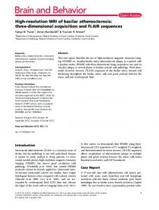
3. Numerical Scheme In this paper, the finite volume method based on the staggered mesh is used to discretize seven conservation equations of the two-pressure model and the semi-implicit solution algorithm using high-resolution TVD schemes is developed to solve such two-pressure model. Figure 1 shows the

4

Science and Technology of Nuclear Installations j−1

j

j+1

g

g

g

K

L+1

L

f

f

Scalar variables: f Volume fraction () Pressures (Pg , Pf ) Specific internal energies (Ug , Uf ) Temperatures (Tg , Tf )

Vector quantities: Phasic velocities ( g , f )

Figure 1: Schematic diagram of the staggered mesh.

staggered mesh schematic. Based on the staggered mesh, the scalar variables such as phasic pressures 𝑃𝑘 , specific internal energies 𝑈𝑘 , phasic temperatures 𝑇𝑘 , and phasic volume fractions 𝛼𝑘 are described at the volume centers and the vector quantities (velocities V𝑘 ) are defined at the volume edges. 3.1. High-Resolution TVD Scheme. Using the convection flux 𝜕(𝛼𝑘 𝜌𝑘 V𝑘 𝐴)/𝜕𝑥 of phasic mass conservation equations and the convection flux 𝜕(𝛼𝑘 𝜌𝑘 𝑈𝑘 V𝑘 𝐴)/𝜕𝑥 of phasic energy conservation equations as examples, these convection fluxes can be, respectively, discretized as 󵄨󵄨 𝜕 󵄨 (𝛼𝑘 𝜌𝑘 V𝑘 𝐴)󵄨󵄨󵄨 󵄨󵄨𝐿 𝜕𝑥 =

𝑛 𝑛 𝑛+1 𝑛 𝑛 𝑛+1 ̇ ̇ ) V𝑘,𝑗 (𝛼̇𝑘,𝑗+1 𝜌𝑘,𝑗+1 𝜌𝑘,𝑗 ) V𝑘,𝑗+1 𝐴 𝑗+1 − (𝛼̇𝑘,𝑗 𝐴𝑗

󵄨󵄨 𝜕 󵄨 (𝛼𝑘 𝜌𝑘 𝑈𝑘 V𝑘 𝐴)󵄨󵄨󵄨 󵄨󵄨𝐿 𝜕𝑥 =

Δ𝑥

,

(11)

𝑛 𝑛 𝑛 𝑛+1 𝑛 𝑛 ̇𝑛 𝑛+1 ̇ ̇ 𝑈𝑘,𝑗 ) V𝑘,𝑗 (𝛼̇𝑘,𝑗+1 𝑈̇ 𝑘,𝑗+1 𝜌𝑘,𝑗+1 𝜌𝑘,𝑗 ) V𝑘,𝑗+1 𝐴 𝑗+1 − (𝛼̇𝑘,𝑗 𝐴𝑗

Δ𝑥

.

It should be noted that the terms 𝑃𝑘 (𝜕/𝜕𝑥)(𝛼𝑘 V𝑘 𝐴) and (𝑃𝑘 − 𝑃int )V𝑘 (𝜕𝛼𝑘 /𝜕𝑥) in energy equations are treated similarly to the convection flux. Order of accuracy for spatial discretization depends significantly on the scheme to calculate the donor quantities with an overdot in numerically evaluated fluxes. There are many numerical methods calculating these quantities; one of the most effective methods is to construct flux limiters based on total variation diminishing (TVD). In this paper, the traditional 1st-order upwind scheme and standard high-order schemes are also discussed for the comparisons with high-resolution flux limiter schemes. ̇ ̇ the For a donor quantity 𝜙 ̇ (this can be 𝛼,̇ 𝜌,̇ 𝛼̇𝜌,̇ or 𝛼̇𝜌𝑈), numerically evaluated general form can be written as [32, 47] 𝜕𝜙 𝑛 Δ𝑥𝐾 { 𝜙𝐾 𝑛 + 𝜓 (𝑟) ( ) , { { { 2 𝜕𝑥 𝑗−1 { 𝜙𝑗𝑛̇ = { { { 𝜕𝜙 𝑛 Δ𝑥𝐿 { {𝜙𝐿 𝑛 − 𝜓 (𝑟) ( ) , 2 𝜕𝑥 𝑗+1 {

if V𝑗 > 0 (12) otherwise

in which 𝜓(𝑟) is termed the flux limiter function and the gradient ratio is given by 𝑛

(𝜕𝜙/𝜕𝑥)𝑗 { { { { 𝑛 , { { { (𝜕𝜙/𝜕𝑥)𝑗−1 𝑟={ 𝑛 { (𝜕𝜙/𝜕𝑥)𝑗 { { { { { 𝑛 , (𝜕𝜙/𝜕𝑥)𝑗+1 {

if V𝑗 > 0 (13) otherwise.

Let 𝜓(𝑟) = 0; the traditional 1st-order upwind scheme (FOU) can be obtained from (12). 𝑛 {𝜙𝐾 , 𝜙𝑗𝑛̇ = { 𝜙 𝑛, { 𝐿

if V𝑗 > 0 otherwise.

(14)

Though FOU scheme is a monotone scheme avoiding nonphysical numerical oscillations, the scheme is of 1st-order accuracy and has significant numerical diffusion resulting in relatively large spatial discretization error. This will be shown in Section 4. Let the limiter function 𝜓(𝑟) be a linear unbounded function; standard high-order linear schemes can be derived from (12), as summarized in Table 1. These linear schemes are of at least 2nd-order accuracy, reducing numerical diffusion effectively, but often lead to unphysical spatial oscillations for the case of sharp gradients which will be shown in the next section. Let the limiter function 𝜓(𝑟) be a bounded function; many researchers [32] have proposed monotonic high-resolution schemes which satisfy TVD [48]; here eight flux limiters are selected, as Table 2 shows. These bounded flux limiter functions are illustrated in Figure 2. All the limiter schemes in Table 2 fulfill TVD and preserve monotonicity to avoid unphysical numerical oscillations under the circumstance of steep gradients. Hereinto, Minmod is the lower bound of second-order TVD region and Superbee is upper bound of second-order TVD region. SMART, Koren, and MUSCL are bounded standard highorder schemes such as QUICK, third-order upwind scheme, and Fromm’s scheme. Harmonic, OSPRE, and Van Albada are symmetric polynomial-ratio schemes.

Science and Technology of Nuclear Installations

5

Table 1: Standard high-order linear schemes for the case of uniform meshes. Scheme name Central-difference scheme (CD)

Limiter function 𝑟

QUICK

3𝑟 + 1 4

Third-order upwind scheme (TOU)

2𝑟 + 1 3

Fromm scheme

𝑟+1 2

Second-order upwind scheme (SOU)

1

Reconstructed variable 𝜙𝑗𝑛̇ =

Property

𝜙𝐾 𝑛 + 𝜙𝐿 𝑛 2

2nd-order accuracy

𝜙𝐾 𝑛 + 𝜙𝐿 𝑛 1 𝑛 { − (𝜙𝐿 − 2𝜙𝐾 𝑛 + 𝜙𝐾−1 𝑛 ), if V𝑗 > 0 { { 2 8 𝑛̇ 𝜙𝑗 = { 𝑛 { 𝜙𝐾 + 𝜙𝐿 𝑛 1 { − (𝜙𝐾 𝑛 − 2𝜙𝐿 𝑛 + 𝜙𝐿+1 𝑛 ), otherwise { 2 8

2nd-order accuracy

𝜙𝐾 𝑛 + 𝜙𝐿 𝑛 1 𝑛 { − (𝜙𝐿 − 2𝜙𝐾 𝑛 + 𝜙𝐾−1 𝑛 ), if V𝑗 > 0 { { 2 6 𝑛̇ 𝜙𝑗 = { 𝑛 𝑛 { 1 { 𝜙𝐾 + 𝜙𝐿 − (𝜙𝐾 𝑛 − 2𝜙𝐿 𝑛 + 𝜙𝐿+1 𝑛 ), otherwise { 2 6

3rd-order accuracy

𝜙𝐾 𝑛 + 𝜙𝐿 𝑛 1 𝑛 { − (𝜙𝐿 − 2𝜙𝐾 𝑛 + 𝜙𝐾−1 𝑛 ), if V𝑗 > 0 { { 2 4 𝑛̇ 𝜙𝑗 = { 𝑛 { 𝜙𝐾 + 𝜙𝐿 𝑛 1 { − (𝜙𝐾 𝑛 − 2𝜙𝐿 𝑛 + 𝜙𝐿+1 𝑛 ), otherwise { 2 4

2nd-order accuracy

3𝜙𝐾 𝑛 − 𝜙𝐾−1 𝑛 { , { { 2 𝜙𝑗𝑛̇ = { 𝑛 𝑛 { { 3𝜙𝐿 − 𝜙𝐿+1 , { 2

2nd-order accuracy

3.2. Semi-Implicit Scheme. RELAP5 code uses some numerical convenient set to overcome serious numerical instabilities associated with gas/liquid phase appearance and disappearance when solving the six-equation single-pressure model [3]. These numerical challenges arise from the degeneration of the model to the single-phase case or opposite resulting in a singular equation system. Similar to RELAP5 [3], for dealing with numerical challenges in phase appearance and disappearance in solving the advanced two-pressure model, mass and momentum conservation equations (1)–(4) are rearranged into sum and difference equation forms and the time derivative terms in conservation equations (1)–(6) are expanded in this numerical scheme. Such semi-implicit scheme is achieved by treating implicitly phasic velocities in mass and energy conservation equations, pressure gradient in momentum conservation equations, and all interfacial exchange terms in conservation equations and all the rest terms are treated effectively at the new time [49, 50]. The time advancement for all conservation equations (1)–(7) is achieved by the first-order approximation. Superscripts “𝑛” and “𝑛 + 1” in the following discretization equations denote the old and new time step, respectively, and subscripts containing “𝐾, 𝐿” determine the spatial position of scalar variables and subscripts containing “𝑗” determine the spatial position of vector variables; the variables with a dot are donor quantities calculated from (12); the variables with an overtilde are the intermediate new time variables that will be corrected in the final. Expanding the time derivative in phasic mass conservation equations (1) and (2) and adding these two expanded mass conservation equations yield the sum mass

if V𝑗 > 0 otherwise

conservation equation. The corresponding finite discretization equation in the control volume 𝐿 can be modeled as 𝑛 𝑛+1 𝑛 𝑛 𝑛+1 𝑛 (𝜌̃𝑔,𝐿 − 𝜌𝑔,𝐿 ) + 𝛼𝑓,𝐿 (𝜌̃𝑓,𝐿 − 𝜌𝑓,𝐿 ) 𝑉𝐿 [𝛼𝑔,𝐿 𝑛 𝑛 𝑛+1 𝑛 + (𝜌𝑔,𝐿 − 𝜌𝑓,𝐿 ) (̃ 𝛼𝑔,𝐿 − 𝛼𝑔,𝐿 )] 𝑛 𝑛 𝑛+1 𝑛 𝑛 𝑛+1 ̇ ̇ V𝑔,𝑗 𝐴 𝑗 ) Δ𝑡 𝜌𝑔,𝑗+1 𝜌𝑔,𝑗 + (𝛼̇𝑔,𝑗+1 V𝑔,𝑗+1 𝐴 𝑗+1 − 𝛼̇𝑔,𝑗

(15)

𝑛 𝑛 𝑛+1 𝑛 𝑛 𝑛+1 ̇ ̇ V𝑓,𝑗 𝐴 𝑗 ) Δ𝑡 = 0 𝜌𝑓,𝑗+1 𝜌𝑓,𝑗 + (𝛼̇𝑓,𝑗+1 V𝑓,𝑗+1 𝐴 𝑗+1 − 𝛼̇𝑓,𝑗

In the same way, expanding the time derivative in the mass conservation equations (1) and (2), subtracting these two expanded mass conservation equations, and substituting (10) for Γ𝑔 yield the difference mass conservation equation. The finite discretization form of the difference mass conservation equation can be given by 𝑛 𝑛+1 𝑛 𝑛 𝑛+1 𝑛 𝑉𝐿 [𝛼𝑔,𝐿 (𝜌̃𝑔,𝐿 − 𝜌𝑔,𝐿 ) − 𝛼𝑓,𝐿 (𝜌̃𝑓,𝐿 − 𝜌𝑓,𝐿 ) 𝑛 𝑛 𝑛+1 𝑛 + (𝜌𝑔,𝐿 + 𝜌𝑓,𝐿 ) (̃ 𝛼𝑔,𝐿 − 𝛼𝑔,𝐿 )] 𝑛 𝑛 𝑛+1 𝑛 𝑛 𝑛+1 ̇ ̇ V𝑔,𝑗 𝐴 𝑗 ) Δ𝑡 + (𝛼̇𝑔,𝑗+1 𝜌𝑔,𝑗+1 𝜌𝑔,𝑗 V𝑔,𝑗+1 𝐴 𝑗+1 − 𝛼̇𝑔,𝑗 𝑛 𝑛 𝑛+1 𝑛 𝑛 𝑛+1 ̇ ̇ V𝑓,𝑗 𝐴 𝑗 ) Δ𝑡 − (𝛼̇𝑓,𝑗+1 𝜌𝑓,𝑗+1 𝜌𝑓,𝑗 V𝑓,𝑗+1 𝐴 𝑗+1 − 𝛼̇𝑓,𝑗 𝑛

2 𝑛 ̃ 𝑠,𝑛+1 − 𝑇 ̃ 𝑛+1 ) = −( ∗ ) 𝑉𝐿 Δ𝑡 [𝐻𝑖𝑔,𝐿 (𝑇 𝐿 𝑔,𝐿 ℎ𝑔 − ℎ𝑓∗ 𝐿

+

𝑛 ̃ 𝑠,𝑛+1 (𝑇 𝐻𝑖𝑓,𝐿 𝐿

̃ 𝑛+1 )] . −𝑇 𝑓,𝐿

(16)

6

Science and Technology of Nuclear Installations Table 2: Flux limiter scheme based on TVD.

Limiter name

Limiter function

Property Lower bound of second-order TVD region [48], bounded central-difference, and second-order upwind scheme

Minmod

max [0, min (𝑟, 1)]

Superbee

max [0, min (2𝑟, 1) , min (𝑟, 2)] 𝑟 + |𝑟| |𝑟| + 1 3𝑟(𝑟 + 1) 2(𝑟2 + 𝑟 + 1) 𝑟(𝑟 + 1) (𝑟2 + 1) 3 1 max [0, min (2𝑟, 𝑟 + , 2)] 4 4 1 2 max [0, min (2𝑟, 𝑟 + , 2)] 3 3 𝑟+1 , 2)] max [0, min (2𝑟, 2

Harmonic OSPRE Van Albada SMART Koren MUSCL

Symmetric polynomial-ratio scheme Symmetric polynomial-ratio scheme Symmetric polynomial-ratio scheme Bounded QUICK scheme Bounded third-order upwind scheme Bounded Fromm’s scheme

The expanded forms of the gas energy equation are defined by expanding the time derivative in gas energy equation (5) and substituting (10). The finite discretization form for the expanded gas energy equation is

2.0

1.5 Limiter function

Upper bound of second-order TVD region [48]

𝑛 𝑛 𝑛 𝑛+1 𝑛 𝑉𝐿 [(𝜌𝑔,𝐿 𝑈𝑔,𝐿 + 𝑃int,𝐿 ) (̃ 𝛼𝑔,𝐿 − 𝛼𝑔,𝐿 )

1.0 𝑛 𝑛 𝑛+1 𝑛 𝑛 𝑛 ̃𝑛+1 − 𝑈𝑛 )] + 𝛼𝑔,𝐿 𝑈𝑔,𝐿 (𝜌̃𝑔,𝐿 − 𝜌𝑔,𝐿 ) + 𝛼𝑔,𝐿 𝜌𝑔,𝐿 (𝑈 𝑔,𝐿 𝑔,𝐿

0.5

𝑛 𝑛 𝑛 𝑛 𝑛+1 ̇ 𝑈̇ 𝑔,𝑗+1 + [𝛼̇𝑔,𝑗+1 (𝜌𝑔,𝑗+1 + 𝑃𝑔,𝐿 ) V𝑔,𝑗+1 𝐴 𝑗+1

0.0 0.0

0.5

1.0

1.5

2.0

2.5

3.0

r Minmod Superbee Harmonic OSPRE

𝑛 𝑛 𝑛+1 𝑛 𝑛 𝑛 ⋅ (𝛼̇𝑔,𝑗+1 − 𝛼𝑔,𝐿 ) V𝑔,𝑗+1 𝐴 𝑗+1 Δ𝑡 − (𝑃𝑔,𝐿 − 𝑃int,𝐿 ) (𝛼̇𝑔,𝑗

Van Albada SMART Koren MUSCL

𝑛 𝑛+1 − 𝛼𝑔,𝐿 ) V𝑔,𝑗 𝐴 𝑗 Δ𝑡

Figure 2: Nonlinear flux limiter functions.

𝑛

By substituting (10) for Γ𝑔 , the finite difference equation for the volume fraction transport equation (7) reads

−

𝑛+1 − 𝑃𝑓,𝐿 )+

(𝛼𝑛𝑔,𝑗

−

𝑛 𝛼̇𝑔,𝐿 )] Δ𝑡

=

𝑛

𝐿

1 𝑛 ̃ 𝑠,𝑛+1 − 𝑇 ̃ 𝑛+1 )] . ) 𝐻𝑖𝑓,𝐿 (𝑇 𝐿 𝑓,𝐿 ℎ𝑔∗ − ℎ𝑓∗ 𝐿

(18)

𝑛

𝑛 ̃ 𝑠,𝑛+1 − 𝑇 ̃ 𝑛+1 ) ) 𝐻𝑖𝑓,𝐿 (𝑇 𝐿 𝑓,𝐿 ℎ𝑔∗ − ℎ𝑓∗ 𝐿

2

+

1 𝑛 𝜌int

𝑛

ℎ𝑔∗

𝑛+1 𝜇𝐿 𝑉𝐿 Δ𝑡 (𝑃𝑔,𝐿

1 𝑛 ̃ 𝑠,𝑛+1 − 𝑇 ̃ 𝑛+1 ) ⋅ 𝑉𝐿 Δ𝑡 [− ( ∗ ) 𝐻𝑖𝑔,𝐿 (𝑇 𝐿 𝑔,𝐿 ℎ𝑔 − ℎ𝑓∗ −(

ℎ𝑓∗ { 𝑛 ̃ 𝑠,𝑛+1 − 𝑇 ̃ 𝑛+1 ) + {− ( ∗ ) 𝐻𝑖𝑔,𝐿 (𝑇 𝐿 𝑔,𝐿 ℎ𝑔 − ℎ𝑓∗ 𝐿 { −(

𝑛+1 𝑛 𝑛+1 𝑛 − 𝛼𝑔,𝐿 ) 𝑉𝐿 + [Vint,𝑗+1 𝐴 𝑗+! (𝛼𝑛𝑔,𝑗+1 − 𝛼̇𝑔,𝐿 ) (̃ 𝛼𝑔,𝐿 𝑛+1 𝐴𝑗 Vint,𝑗

𝑛 𝑛 𝑛 𝑛 𝑛+1 𝑛 𝑛 ̇ 𝑈̇ 𝑔,𝑗 − 𝛼̇𝑔,𝑗 (𝜌𝑔,𝑗 + 𝑃𝑔,𝐿 ) V𝑔,𝑗 𝐴 𝑗 ] Δ𝑡 = (𝑃𝑔,𝐿 − 𝑃int,𝐿 )

𝑛 Γ𝑔,𝐿 (

(V𝑔 − Vint ) 2

𝑛

) 𝐿

(17) 𝑛

} 1 𝑓wall,𝑔 󵄨 󵄨 +( 𝜌 V2 󵄨󵄨󵄨V 󵄨󵄨󵄨 𝛼 ) 𝑉 Δ𝑡. 2 𝐷 𝑔 𝑔 󵄨 𝑔 󵄨 𝑔 𝐿} 𝐿 } Expanding the time derivative in liquid energy equation (6) and substituting (10) yield the expanded liquid energy

Science and Technology of Nuclear Installations

7

equation. The finite discretization form for the expanded liquid energy equation is expressed as 𝑛 𝑛 𝑛 𝑛+1 𝑛 𝑉𝐿 [− (𝜌𝑓,𝐿 𝑈𝑓,𝐿 + 𝑃int,𝐿 ) (̃ 𝛼𝑔,𝐿 − 𝛼𝑔,𝐿 )

𝑛

𝑗

𝑛 𝑛 𝑛 𝑛 𝑛+1 ̇ 𝑈̇ 𝑓,𝑗+1 (𝜌𝑓,𝑗+1 + 𝑃𝑓,𝐿 ) V𝑓,𝑗+1 𝐴 𝑗+1 + [𝛼̇𝑓,𝑗+1

+

𝑛 𝑛 𝑛 𝑛 𝑛+1 𝑛 𝑛 ̇ 𝑈̇ 𝑓,𝑗 − 𝛼̇𝑓,𝑗 (𝜌𝑓,𝑗 + 𝑃𝑓,𝐿 ) V𝑓,𝑗 𝐴 𝑗 ] Δ𝑡 = (𝑃𝑓,𝐿 − 𝑃int,𝐿 )

𝑛 − Γ𝑔,𝐿 (

(19)

𝑛

) 𝐿

} 1 𝑓𝑤𝑎𝑙𝑙,𝑘 󵄨 󵄨 𝜌𝑓 V𝑓2 󵄨󵄨󵄨󵄨V𝑓 󵄨󵄨󵄨󵄨 𝛼𝑓 ) } 𝑉𝐿 Δ𝑡. 2 𝐷 𝐿 }

Momentum equations (3)-(4) are firstly rearranged into the expanded forms by substituting mass conservation equations (1)-(2). 𝛼𝑔 𝜌𝑔 𝐴

𝜕V𝑔 𝜕𝑡

= −𝛼𝑔 𝐴

+ 𝛼𝑔 𝜌𝑔 V𝑔 𝐴 𝜕𝑃𝑔 𝜕𝑥

𝜕V𝑔

+ (𝑃int − 𝑃𝑔 ) 𝐴

𝜕𝛼𝑔

𝜕𝑡

= −𝛼𝑓 𝐴

+ 𝛼𝑓 𝜌𝑓 V𝑓 𝐴 𝜕𝑃𝑓 𝜕𝑥

[(V𝑔𝑛+1 − V𝑔𝑛 ) − (V𝑓𝑛+1 − V𝑓𝑛 )] Δ𝑥𝑗 + 𝑗

𝜕𝑥

𝐾

+ 𝛼𝑔 𝜌𝑔 𝑔𝑥 𝐴 (20)

𝑛

𝑛 𝑛 1 1 [(V𝑓2 ) − (V𝑓2 ) ] Δ𝑡 = − ( ) 𝐿 𝐾 2 𝜌𝑔 𝑗

𝑛+1 𝑛+1 ⋅ (𝑃𝑔,𝐿 − 𝑃𝑔,𝐾 ) Δ𝑡 + (

𝑛

1 𝑛+1 ) (𝑃𝑛+1 − 𝑃𝑓,𝐾 ) Δ𝑡 𝜌𝑓 𝑗 𝑓,𝐿

𝑛

𝑛+1 𝑛+1 𝑛 𝑛 − 𝑃𝑔,𝐾 ) (𝛼𝑔,𝐾 − 𝛼𝑔,𝑗 )] − ( − (𝑃int,𝐾

𝜕V𝑓 𝑛+1 𝑛+1 𝑛 𝑛 ⋅ Δ𝑡 [(𝑃int,𝐿 − 𝑃𝑓,𝐿 ) (𝛼𝑓,𝐿 − 𝛼𝑓,𝑗 )

𝜕𝑥

+ (𝑃int − 𝑃𝑓 ) 𝐴

𝜕𝛼𝑓 𝜕𝑥

𝑛+1 𝑛+1 𝑛 𝑛 − 𝑃𝑓,𝐾 ) (𝛼𝑓,𝐾 − 𝛼𝑓,𝑗 )] − (𝑃int,𝐾

+ 𝛼𝑓 𝜌𝑓 𝑔𝑥 𝐴

− Γ𝑔 (Vint − V𝑓 ) 𝐴 1 󵄨 󵄨 + 𝜌𝑐 𝐶𝑖𝐷𝐴 int (V𝑔 − V𝑓 ) 󵄨󵄨󵄨󵄨V𝑔 − V𝑓 󵄨󵄨󵄨󵄨 𝐴 8 1 𝑓wall,𝑓 󵄨 󵄨 − 𝜌𝑓 V𝑓 󵄨󵄨󵄨󵄨V𝑓 󵄨󵄨󵄨󵄨 𝛼𝑓 𝐴. 2 𝐷

𝑛 1 [(V𝑔2 ) 𝐿 2

1 𝑛+1 𝑛+1 𝑛 𝑛 ) Δ𝑡 [(𝑃int,𝐿 − 𝑃𝑔,𝐿 ) (𝛼𝑔,𝐿 − 𝛼𝑔,𝑗 ) +( 𝛼𝑔 𝜌𝑔 𝑗

1 𝑓wall,𝑔 󵄨 󵄨 𝜌 V 󵄨󵄨󵄨V 󵄨󵄨󵄨 𝛼 𝐴, 2 𝐷 𝑔 𝑔 󵄨 𝑔󵄨 𝑔

𝜕V𝑓

The difference momentum equation is obtained by dividing gas momentum equation (20) by 𝛼𝑔 𝜌𝑔 𝐴 and dividing liquid momentum equation (21) by 𝛼𝑓 𝜌𝑓 𝐴, respectively, and subtracting them. The finite difference equation for the difference momentum equation can be written as

𝑛

1 󵄨 󵄨 − 𝜌𝑐 𝐶𝑖𝐷𝐴 int (V𝑔 − V𝑓 ) 󵄨󵄨󵄨󵄨V𝑔 − V𝑓 󵄨󵄨󵄨󵄨 𝐴 8

𝛼𝑓 𝜌𝑓 𝐴

𝑛+1

− (V𝑔2 ) ] Δ𝑡 −

𝜕𝑥

+ Γ𝑔 (Vint − V𝑔 ) 𝐴

−

𝑛+1 1 𝑓wall,𝑓 󵄨 󵄨 𝜌𝑓 𝛼𝑓 󵄨󵄨󵄨󵄨V𝑓 󵄨󵄨󵄨󵄨) (V𝑓 )𝑗 2 𝐷 𝑗

− (Γ𝑔 )𝑗 (V𝑔 − V𝑓 )𝑗 ] Δ𝑥𝑗 Δ𝑡.

𝑛

2

𝑛

+(

(22)

𝑛

𝐿

2

𝐾

𝑛+1 1 𝑓wall,𝑔 󵄨 󵄨 −( 𝜌𝑔 𝛼𝑔 󵄨󵄨󵄨󵄨V𝑔 󵄨󵄨󵄨󵄨) (V𝑔 )𝑗 2 𝐷 𝑗

−(

𝑛 ̃ 𝑠,𝑛+1 − 𝑇 ̃ 𝑛+1 ) ) 𝐻𝑖𝑓,𝐿 (𝑇 𝐿 𝑓,𝐿

(V𝑓 − Vint )

𝑛

𝐿

𝑛

𝑛

ℎ𝑔∗ − ℎ𝑓∗

𝑛

𝑛

𝑛

{ 𝑛 ̃ 𝑠,𝑛+1 − 𝑇 ̃ 𝑛+1 ) ) 𝐻𝑖𝑔,𝐿 (𝑇 + {( ∗ 𝐿 𝑔,𝐿 ℎ𝑔 − ℎ𝑓∗ 𝐿 { +(

𝑛 𝑛 𝑛 𝑛 1 1 (𝛼 𝜌 ) [(V𝑔2 ) − (V𝑔2 ) ] Δ𝑡 + (𝛼𝑓 𝜌𝑓 )𝑗 𝐿 𝐾 2 𝑔 𝑔 𝑗 2

𝑛 𝑛+1 𝑛 𝑛+1 − (𝛼𝑓,𝐿 𝑃𝑓,𝐿 − 𝛼𝑓,𝐾 𝑃𝑓,𝐾 ) Δ𝑡 + [(𝜌𝑚 )𝑗 𝑔𝑥

𝑛 𝑛+1 𝛼𝑓,𝐿 ) V𝑓,𝑗 𝐴 𝑗 Δ𝑡

ℎ𝑔∗

𝑗

𝑛 𝑛+1 𝑛 𝑛+1 ⋅ [(V𝑓2 ) − (V𝑓2 ) ] Δ𝑡 = − (𝛼𝑔,𝐿 𝑃𝑔,𝐿 − 𝛼𝑔,𝐾 𝑃𝑔,𝐾 ) Δ𝑡

𝑛 𝑛 𝑛+1 𝑛 𝑛 𝑛 − 𝛼𝑓,𝐿 ) V𝑓,𝑗+1 𝐴 𝑗+1 Δ𝑡 − (𝑃𝑓,𝐿 − 𝑃int,𝐿 ) (𝛼̇𝑓,𝑗 ⋅ (𝛼̇𝑓,𝑗+1

ℎ𝑓∗

𝑛

(𝛼𝑔 𝜌𝑔 )𝑗 (V𝑔𝑛+1 − V𝑔𝑛 ) Δ𝑥𝑗 + (𝛼𝑓 𝜌𝑓 )𝑗 (V𝑓𝑛+1 − V𝑓𝑛 ) Δ𝑥𝑗

𝑛 𝑛 𝑛+1 𝑛 𝑛 𝑛 ̃𝑛+1 − 𝑈𝑛 )] 𝑈𝑓,𝐿 (𝜌̃𝑓,𝐿 − 𝜌𝑓,𝐿 ) + 𝛼𝑓,𝐿 𝜌𝑓,𝐿 (𝑈 + 𝛼𝑓,𝐿 𝑓,𝐿 𝑓,𝐿

−

Adding (20) and (21) yields the sum momentum equation. The sum momentum equation can be converted into the following discretization form.

(21)

{ { 1 𝑓wall,𝑔 − {( { 2 𝐷 { 1 𝑓wall,𝑓 −( 2 𝐷

𝑛

𝑛+1 󵄨󵄨 󵄨󵄨 󵄨󵄨V𝑔 󵄨󵄨) (V𝑔 ) 󵄨 󵄨 𝑗 𝑗

𝑛

𝑛+1 󵄨󵄨 󵄨󵄨 󵄨󵄨V𝑓 󵄨󵄨) (V𝑓 ) 󵄨 󵄨 𝑗 𝑗

𝑛

1 ) 𝛼𝑓 𝜌𝑓 𝑗

8

Science and Technology of Nuclear Installations −[ [

𝑛+1 − 𝛼𝑓𝑛 𝜌𝑓𝑛 V𝑔𝑛+1 − 𝛼𝑔𝑛 𝜌𝑔𝑛 V𝑓𝑛+1 ) Γ𝑔𝑛 (𝜌𝑚𝑛 Vint

(𝛼𝑔 𝜌𝑔 𝛼𝑓 𝜌𝑓 )

𝑛

linear algebraic equation set with 7𝑁 unknown solution variables which can be solved by Gauss elimination solver [51]. ̃𝑛+1 , and 𝛼̃𝑛+1 are ̃𝑛+1 , 𝑈 The intermediate new time variables 𝑈 𝑔 𝑓 𝑔 solved by expanded time derivative forms of conservation equations such that there are linearization errors in these solutions. To alleviate these errors, the final 𝑈𝑔𝑛+1 , 𝑈𝑓𝑛+1 , and 𝛼𝑔𝑛+1 are solved again by unexpanded forms of mass and ̃𝑛+1 , and 𝛼̃𝑛+1 ̃𝑛+1 , 𝑈 energy conservation equations where 𝑈 𝑔 𝑓 𝑔 are used for evaluation of the source terms of conservation equations, similar to RELAP5 [49].

] ]𝑗

𝑛

+(

𝜌𝑚 1 󵄨 󵄨 ⋅ 𝜌 𝐶 𝐴 󵄨󵄨󵄨V − V𝑓 󵄨󵄨󵄨󵄨) 𝛼𝑔 𝜌𝑔 𝛼𝑓 𝜌𝑓 8 𝑐 𝑖𝐷 int 󵄨 𝑔 𝑗

} } ⋅ (V𝑔𝑛+1 − V𝑓𝑛+1 ) } Δ𝑥𝑗 Δ𝑡. 𝑗} } (23) A variable with an overbar is calculated as an averaged quantity in the following. 𝜙𝑗 =

𝜙𝐾 Δ𝑥𝐾 + 𝜙𝐿 Δ𝑥𝐿 . Δ𝑥𝐾 + Δ𝑥𝐿

(24)

In order to close the system, equations of state for water properties are supplemented. The properties are based on IAPWS IF-97. In this paper, phasic densities and temperatures are provided as functions of phasic pressures or/and phasic specific internal energies and the linearized equations of state are given as 𝑛+1 𝑛 = 𝜌𝑔,𝐿 +( 𝜌̃𝑔,𝐿

+(

𝜕𝑃𝑔

+(

𝐿

𝜕𝜌𝑓 𝜕𝑃𝑓

𝑛

𝑛+1 𝑛 ) (𝑃𝑓,𝐿 − 𝑃𝑓,𝐿 ) 𝐿

𝑛

𝜕𝜌𝑓 𝜕𝑈𝑓

̃𝑛+1 − 𝑈𝑛 ) , ) (𝑈 𝑓,𝐿 𝑓,𝐿 𝐿

𝜕𝑇𝑔 𝜕𝑃𝑔

𝑛

𝑛+1 𝑛 ) (𝑃𝑔,𝐿 − 𝑃𝑔,𝐿 )

(25)

𝐿

𝑛

𝜕𝑇𝑔 𝜕𝑈𝑔

̃ 𝑛+1 = 𝑇𝑛 + ( 𝑇 𝑓,𝐿 𝑓,𝐿

𝐿

̃𝑛+1 − 𝑈𝑛 ) , ) (𝑈 𝑔,𝐿 𝑔,𝐿

𝜕𝑈𝑔

̃ 𝑛+1 = 𝑇𝑛 + ( 𝑇 𝑔,𝐿 𝑔,𝐿 +(

𝑛

𝑛+1 𝑛 ) (𝑃𝑔,𝐿 − 𝑃𝑔,𝐿 )

𝑛

𝜕𝜌𝑔

𝑛+1 𝑛 𝜌̃𝑓,𝐿 = 𝜌𝑓,𝐿 +(

+(

𝜕𝜌𝑔

̃𝑛+1 − 𝑈𝑛 ) , ) (𝑈 𝑔,𝐿 𝑔,𝐿 𝐿

𝜕𝑇𝑓 𝜕𝑃𝑓

𝜕𝑇𝑓 𝜕𝑈𝑓

𝑛

𝑛+1 𝑛 ) (𝑃𝑓,𝐿 − 𝑃𝑓,𝐿 ) 𝐿

𝑛

̃𝑛+1 − 𝑈𝑛 ) , ) (𝑈 𝑓,𝐿 𝑓,𝐿 𝐿

𝑛

𝑠 ̃ 𝑠,𝑛+1 = 𝑇𝑠,𝑛 + ( 𝜕𝑇 ) (𝑃𝑛+1 − 𝑃𝑛 ) . 𝑇 𝐿 𝐿 int,𝐿 𝜕𝑃int 𝐿 int,𝐿

On substituting directly (25) into these seven discretization equations (15)–(19) and (22)-(23), seven discretization equations correspond to seven unknown solution variables (𝛼𝑔 , 𝑃𝑔 , 𝑃𝑓 , 𝑈𝑔 , 𝑈𝑓 , V𝑔 , and V𝑓 ). For a system containing 𝑁 volumes, these seven discretization equations form a 7𝑁

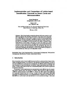
4. Numerical Test In this section, the water faucet problem is simulated to assess the proposed solution scheme based on two-pressure model. Here, high-resolution TVD schemes are implemented in such scheme to demonstrate the high-order of spatial accuracy. For comparisons, results from traditional 1st-order upwind scheme and classical high-order linear schemes are shown. 4.1. Water Faucet Problem. The water faucet problem proposed by Ransom [52] is one of the most important benchmark tests for validating the ability of numerical scheme to calculate two-phase flows. The geometric configuration is a vertical tube of 12 m in length with the diameter of 1 m. Initially, the tube is composed of a uniform annulus of gas with initial velocity V𝑔,initial = 0 m/s and a surrounded uniform column of water with initial velocity V𝑓,initial = 10 m/s. The initial gas volume fraction is 0.2 and all the initial phasic pressures are set to 0.1 MPa. The wall and interfacial drags are ignored and no phase transition is assumed; then the flow goes down driven by the gravity. A schematic diagram of the time evolution for this water faucet problem is shown in Figure 3. Based on the above initial conditions and assumptions, analytical solutions for the gas volume fraction and liquid velocity distribution with time along the pipe length direction have been obtained and are given in the following [53, 54]. 𝛼𝑔 (𝑥, 𝑡) (1 − 𝛼𝑔,initial ) V𝑓,initial 𝑡2 { { , 𝑥 ≤ V𝑓,initial 𝑡 + 𝑔𝑥 {1 − 2 2 ={ + 2𝑔𝑥 𝑥 √V𝑓,initial { { otherwise, {𝛼𝑔,initial , 𝑡2 2 { + 2𝑔𝑥 𝑥, 𝑥 ≤ V𝑓,initial 𝑡 + 𝑔𝑥 {√V𝑓,initial 2 V𝑓 (𝑥, 𝑡) = { { otherwise. {V𝑓,initial + 𝑔𝑥 𝑡,

(26)

(27)

The gravity accelerates the rate of the liquid; then the liquid column becomes thinner with time; there is a moving discontinuity in the profile (see Figure 3), where it is a very important region for testing the accuracy of the numerical scheme and its stability near discontinuities. All the following numerical results are calculated using a fixed initial liquid Courant number of CFL𝑓 = 0.2. Numerical simulations using the classical FOU scheme are performed

Science and Technology of Nuclear Installations

9 18

Inlet

17 Liquid velocity (m/s)

16

Gravity

15 14 13 12 11 10 9 0

Outlet

Time

Figure 3: Illustration of the time evolution for the faucet flow problem.

2

4

6 x (m)

8

10

12

Analytical solution, t = 0.2 s Numerical solution, 96 cells, t = 0.2 s Analytical solution, t = 0.5 s Numerical solution, 96 cells, t = 0.5 s Analytical solution, t = 0.75 s Numerical solution, 96 cells, t = 0.75 s

Figure 5: Numerical results from FOU scheme with 96 cells of liquid velocity compared with analytical results at time of 0.2, 0.5, and 0.75 seconds.

0.55

Gas volume fraction

0.50 0.45 0.40 0.35 0.30 0.25 0.20 0.15 0

2

4

6 x (m)

8

10

12

Analytical solution, t = 0.2 s Numerical solution, 96 cells, t = 0.2 s Numerical solution, 192 cells, t = 0.2 s Analytical solution, t = 0.5 s Numerical solution, 96 cells, t = 0.5 s Numerical solution, 192 cells, t = 0.5 s Analytical solution, t = 0.75 s Numerical solution, 96 cells, t = 0.75 s Numerical solution, 192 cells, t = 0.75 s

Figure 4: Gas volume fraction comparison between analytical solutions and numerical solutions from FOU scheme with 96 cells and 192 cells at time of 0.2, 0.5, and 0.75 seconds.

first. Figure 4 shows results of gas volume fraction distribution with 96 cells and 192 cells at times 0.2, 0.5, and 0.75 s. This figure illustrates the numerical stability to handle discontinuities and the numerical results are excellently consistent with the corresponding analytical solutions except the near discontinuities (𝑥 = V𝑓,initial 𝑡 + 𝑔𝑥 𝑡2 /2). The difference near

discontinuities between numerical and analytical solutions is caused by the numerical diffusion from the FOU scheme. As shown in this figure, the numerical results with 192 cells are more accurate than those with 96 cells which means that the finer the grid is, the smaller the numerical diffusion is. However finer meshes require more computation time and decrease the efficiency; high-order schemes are needed to reduce numerical errors more effectively. The numerical results with 96 cells of liquid velocity distribution are presented in Figure 5. It can be observed that the calculated liquid velocities are in very good agreement with the corresponding analytical solutions such that the calculated results with 192 cells are not given in this figure. Furthermore, finer grid FOU resolutions ranging from 384 to 1152 cells are studied with single-pressure model and two-pressure model, as shown in Figures 6 and 7, and the comparisons of them are shown in Figure 8. For the case of 1152 cells, numerical solutions of single-pressure model show a big undershoot at the discontinuity which is due to the nature of ill-posedness. As compared to single-pressure model, numerical solutions of two-pressure model are more stable under the same conditions. Secondly, numerical simulations using standard highorder linear schemes (Table 1) are performed with 96 cells. Figure 9 shows the gas volume fraction distribution using standard high-order linear schemes at 0.75 s. For the comparisons, the result from FOU scheme is also shown in the figure (dash line). It is observed that, as compared to FOU scheme, standard high-order linear schemes reduce the numerical dissipation effectively and TOU scheme seems to be more accurate than other standard high-order linear schemes due to its 3rd-order precision. But unphysical oscillation occurs

Science and Technology of Nuclear Installations 0.5

0.5

0.4

0.4 Gas volume fraction

Gas volume fraction

10

0.3

0.2

0.3

0.2

0.1

0.1

0.0

0.0 0

2

4

6 Distance (m)

8

10

5.0 5.2 5.4 5.6 5.8 6.0 6.2 6.4 6.6 6.8 7.0 7.2 7.4 Distance (m)

12

Single-pressure model, 384 cells, CFL = 0.2 Single-pressure model, 768 cells, CFL = 0.2 Single-pressure model, 1152 cells, CFL = 0.2 Two-pressure model, 384 cells, CFL = 0.2 Two-pressure model, 768 cells, CFL = 0.2 Two-pressure model, 1152 cells, CFL = 0.2 Analytical solution, t = 0.5 s

Single-pressure model, 384 cells, CFL = 0.2 Single-pressure model, 768 cells, CFL = 0.2 Single-pressure model, 1152 cells, CFL = 0.2 Analytical solution, t = 0.5 s

Figure 6: Numerical results of gas volume fraction using singlepressure model and FOU scheme with finer cells at time of 0.5 seconds.

Figure 8: Gas volume fraction comparison between single-pressure model and two-pressure model with FOU scheme and finer cells at time of 0.5 seconds.

0.50 0.6 0.5

0.40 Gas volume fraction

Gas volume fraction

0.45

0.35 0.30 0.25

0.4 0.3 0.2

0.20 0.1 0.15 0

2

4

6 Distance (m)

8

10

12

Two-pressure model, 384 cells, CFL = 0.2 Two-pressure model, 768 cells, CFL = 0.2 Two-pressure model, 1152 cells, CFL = 0.2 Analytical solution, t = 0.5 s

Figure 7: Numerical results of gas volume fraction using twopressure model and FOU scheme with finer cells at time of 0.5 seconds.

near discontinuities in some schemes (TOU, Fromm, CD, and SOU scheme). This oscillation can be explained by Godunov’s order barrier theorem [33] which states that linear unbounded high-order schemes used to solve the advection equation are not monotonic, allowing unphysical oscillations under some circumstances such as this case of discontinuities. To achieve monotonic high-order schemes,

0.0 0

2

4

Analytical solution, t = 0.75 s FOU CD QUICK

6 X (m)

8

10

12

TOU Fromm SOU

Figure 9: Gas volume fraction comparison between analytical solutions and numerical solutions using standard high-order linear schemes with 96 cells at time of 0.75 seconds.

constructing bounded flux limiters based on TVD is one of the most effective methods. Some flux limiters are piecewiselinear functions constructed from bounded standard highorder linear schemes without compromising their high-order precision as shown in Figure 9.

Science and Technology of Nuclear Installations

11 Table 3: Order of accuracy for the TVD scheme.

0.55

Limiter name Superbee Koren MUSCL SMART Harmonic OSPRE Van Albada Minmod FOU

Gas volume fraction

0.50 0.45 0.40 0.35 0.30 0.25 0.20 0

2

4

Analytical solution, t = 0.75 s FOU MUSCL Minmod Superbee

6 X (m)

8

10

12

Harmonic OSPRE Van Albada SMART Koren

5. Conclusions

Figure 10: Gas volume fraction comparison between analytical solutions and numerical solutions using high-resolution TVD schemes with 96 cells at time of 0.75 seconds.

Finally, eight high-resolution TVD schemes in Table 2 are analyzed with 96 cells. Figure 10 shows the gas volume fraction distribution using high-resolution TVD schemes at 0.75 s and results for various high-resolution TVD schemes are presented in Figure 11, respectively. All of the flux limiter schemes have effectively reduced numerical diffusion and improved the prediction of gas volume fraction. As expected, when compared to unstable results from unbounded SOU, TOU, CD, and Fromm scheme, the corresponding bounded TVD schemes Minmod, Koren, and MUSCL produce stable and more accurate results. Among all the flux limiter schemes, Minmod performs worst to reduce numerical diffusion at the discontinuity point 𝑥 = V𝑓,initial 𝑡 + 𝑔𝑥 𝑡2 /2. Results from Superbee seem to be more accurate than those from the other seven schemes at the discontinuity point. In order to analyze the order of accuracy of considered high-resolution schemes, L1 norm of errors between the numerical results and exact solutions on gas volume fraction is assessed and given as 𝐿 1 (𝛼) =

1 𝑁 󵄨󵄨 󵄨 ∑ 󵄨󵄨󵄨𝛼𝑔,numerical (𝑥𝑖 ) − 𝛼𝑔,exact (𝑥𝑖 )󵄨󵄨󵄨󵄨 , 𝑁 𝑖=1

L1 error 0.00605 0.007609 0.008085 0.008143 0.009161 0.00948 0.009977 0.011765 0.02383

(28)

where 𝑁 is the number of control volumes in the domain; here 𝑁 = 96; 𝛼numerical (𝑥𝑖 ) is the numerical solution at 𝑥𝑖 and 𝛼exact (𝑥𝑖 ) is the exact solution from (26) at 𝑥𝑖 . Table 3 shows the order of decreasing accuracy for the TVD schemes. Obviously, Superbee is the most accurate scheme while Minmod is more smeared than other schemes. Koren performs the second best due to a bounded third-order upwind scheme based on TVD.

In this paper, a semi-implicit numerical algorithm based on the finite volume method associated with staggered grids has been developed to solve the advanced well-posed twofluid seven-equation two-pressure model. To overcome the challenge of excessive numerical diffusion from FOU scheme, eight high-resolution TVD schemes are implemented in such numerical algorithm to improve spatial accuracy. Then such new numerical algorithm is validated on the water faucet test, demonstrating high-order spatial accuracy of TVD schemes and robustness near discontinuities. Numerical comparisons reveal that Superbee and Koren give two highest levels of accuracy while Minmod seems to be the worst scheme as compared to other schemes. This research will lay the foundation for more accurately simulating two-phase flows based on the two-pressure model with higher fidelity algorithm.

Nomenclature Symbol Gas density (kg⋅m−3 ) Liquid density (kg⋅m−3 ) Gas velocity (m⋅s−1 ) Liquid velocity (m⋅s−1 ) The cross-sectional area in the pipeline (m2 ) The net gas-liquid mass transfer Γ𝑔 : per unit volume (kg⋅m−3 ⋅s−1 ) Gas pressure (Pa) 𝑃𝑔 : Liquid pressure (Pa) 𝑃𝑓 : 𝑃int : Interfacial pressure (Pa) The gravity acceleration (m⋅s−2 ) 𝑔𝑥 : Vint : The interfacial velocity (m⋅s−1 ) 𝑓wall,𝑘 : The wall friction coefficient for phase 𝑘 𝐷: The hydraulic diameter (m) 𝐴 int : The interfacial area between two phases per unit volume (m−1 ) The continuous phase density (kg⋅m−3 ) 𝜌𝑐 : 𝐶𝑖𝐷: The interfacial drag coefficient between two phases 𝜌𝑔 : 𝜌𝑓 : V𝑔 : V𝑓 : 𝐴:

Science and Technology of Nuclear Installations 0.55

0.55

0.50

0.50

Gas volume fraction

Gas volume fraction

12

0.45 0.40 0.35 0.30 0.25 0.20

0.45 0.40 0.35 0.30 0.25 0.20

0

2

4

6 X (m)

8

10

12

0

0.55

0.50

0.50

Gas volume fraction

Gas volume fraction

0.55 0.45 0.40 0.35 0.30 0.25 0.20

6 X (m)

8

10

12

0.45 0.40 0.35 0.30 0.25 0.20

0

2

4

6 X (m)

8

10

12

0

2

4

6 X (m)

8

10

12

Analytical solution, t = 0.75 s FOU Harmonic

Analytical solution, t = 0.75 s FOU Superbee 0.55

0.55

0.50

0.50

Gas volume fraction

Gas volume fraction

4

Analytical solution, t = 0.75 s FOU Minmod

Analytical solution, t = 0.75 s FOU MUSCL

0.45 0.40 0.35 0.30 0.25

0.45 0.40 0.35 0.30 0.25 0.20

0.20 0

2

4

6 X (m)

8

10

12

0

2

4

6

8

10

12

X (m)

Analytical solution, t = 0.75 s FOU OSPRE

Analytical solution, t = 0.75 s FOU Van Albada

0.55

0.55

0.50

0.50

Gas volume fraction

Gas volume fraction

2

0.45 0.40 0.35 0.30 0.25 0.20

0.45 0.40 0.35 0.30 0.25 0.20

0

2

4

6 X (m)

8

10

Analytical solution, t = 0.75 s FOU SMART

12

0

2

4

6 X (m)

8

10

12

Analytical solution, t = 0.75 s FOU Koren

Figure 11: Numerical solutions of gas volume fraction for various high-resolution TVD schemes at time of 0.75 seconds.

Science and Technology of Nuclear Installations

13

𝑈𝑔 : Vapor/gas specific internal energy (J⋅kg−1 ) 𝑈𝑓 : Liquid specific internal energy (J⋅kg−1 ) 𝐻𝑖𝑔 : Interface-to-gas convective heat transfer coefficient per unit volume (W⋅m−3 ⋅K−1 ) 𝐻𝑖𝑓 : Interface-to-liquid convective heat transfer coefficient per unit volume (W⋅m−3 ⋅K−1 ) 𝑇𝑘 : Temperature for phase 𝑘 (K) 𝑇𝑠 : The saturation temperature under the interfacial pressure 𝑃int (K) ℎ𝑔∗ : The gas specific enthalpy evaluated at the interfacial mass transfer condition (J⋅kg−1 ) ∗ ℎ𝑓 : The liquid specific enthalpy evaluated at the interfacial mass transfer condition (J⋅kg−1 ) 𝜇: The pressure relaxation coefficient function (Pa−1 ⋅s−1 ) 𝜌int : The interfacial density corresponding to the liquid saturated density with 𝑃int (kg⋅m−3 ) 𝑍𝑘 : The phase 𝑘 acoustic impedance (kg⋅m−2 ⋅s−1 ) 𝑐𝑘 : The phase 𝑘 sound velocity (m⋅s−1 ) Δ𝑥: The length of the control volume (m) 𝑉𝐿 : Volume of the control cell 𝐿 (m3 ) 𝑁: Number of control volumes in a system.

of the 8th International Symposium on Symbiotic Nuclear Power Systems for 21st Century, Chengdu, China, 2016. M. R. Baer and J. W. Nunziato, “A two-phase mixture theory for the deflagration-to-detonation transition (ddt) in reactive granular materials,” International Journal of Multiphase Flow, vol. 12, no. 6, pp. 861–889, 1986. R. A. Berry, R. Saurel, and O. LeMetayer, “The discrete equation method (DEM) for fully compressible, two-phase flows in ducts of spatially varying cross-section,” Nuclear Engineering and Design, vol. 240, no. 11, pp. 3797–3818, 2010. R. A. Berry, R. Saurel, F. Petitpas et al., “Progress in the Development of Compressible, Multiphase Flow Modeling Capability for Nuclear Reactor Flow Applications,” Tech. Rep. INL/EXT08-15002, 2008. A. Chinnayya, E. Daniel, and R. Saurel, “Modelling detonation waves in heterogeneous energetic materials,” Journal of Computational Physics, vol. 196, no. 2, pp. 490–538, 2004. H. Lim, U. Lee, K. Kim, and W. J. Lee, “Application of Hyperbolic Two-fluids Equations to Reactor Safety Code,” Nuclear Engineering Technology, vol. 35, 2003. J. H. Song and M. Ishii, “The well-posedness of incompressible one-dimensional two-fluid model,” International Journal of Heat and Mass Transfer, vol. 43, no. 12, pp. 2221–2231, 2000. R. Saurel and R. Abgrall, “A multiphase Godunov method for compressible multifluid and multiphase flows,” Journal of Computational Physics, vol. 150, no. 2, pp. 425–467, 1999. Y. Chen, J. Glimm, D. H. Sharp, and Q. Zhang, “A two-phase flow model of the Rayleigh–Taylor mixing zone,” Physics of Fluids, vol. 8, no. 3, pp. 816–825, 1996. V. H. Ransom and D. L. Hicks, “Hyperbolic two-pressure models for two-phase flow,” Journal of Computational Physics, vol. 53, no. 1, pp. 124–151, 1984. V. H. Ransom and M. P. Scofield, “Two-pressure hydrodynamic model for two-phase separated flow,” SRD-50-76, Idaho National Engineering Laboratory, 1976. J. Hadamard, Lectures on Cauchy’s Problem in Linear Partial Differential Equations, Dover Publications, New York, NY, USA, Primary Source Edition edition, 2014. R. A. Berry, J. W. Peterson, H. Zhang et al., “Relap-7 theory manual, Idaho National Laboratory,” Tech. Rep. INL/EXT-14, 31366, Idaho National Laboratory, 2014. A. Guelfi, D. Bestion, M. Boucker et al., “NEPTUNE: a new software platform for advanced nuclear thermal hydraulics,” Nuclear Science and Engineering, vol. 156, no. 3, pp. 281–324, 2007. R. Szilard, D. Kothe, and P. Turinsky, The Consortium for Advanced Simulation of Light Water Reactors, Enlarged Halden Programme Group Meeting, Sandefjord, Norway, 2011. P. Emonot, A. Souyri, J. L. Gandrille, and F. Barr´e, “CATHARE3: A new system code for thermal-hydraulics in the context of the NEPTUNE project,” Nuclear Engineering and Design, vol. 241, no. 11, pp. 4476–4481, 2011. S. Liang, W. Liu, and L. Yuan, “Solving seven-equation model for compressible two-phase flow using multiple GPUs,” Computers & Fluids, vol. 99, pp. 156–171, 2014. A. Zein, M. Hantke, and G. Warnecke, “Modeling phase transition for compressible two-phase flows applied to metastable liquids,” Journal of Computational Physics, vol. 229, no. 8, pp. 2964–2998, 2010. T. Gallou¨et, J.-M. H´erard, and N. Seguin, “Numerical modeling of two-phase flows using the two-fluid two-pressure approach,”

Subscript/Superscript 𝑔: 𝑓: int: 𝑘: Initial:

Gas phase Liquid phase Phasic interface Gas phase (𝑔) or liquid phase (𝑓) Initial condition.

Conflicts of Interest

[5]

[6]

[7]

[8]

[9]

[10]

[11]

[12]

[13]

[14]

[15]

[16]

The authors declare that they have no conflicts of interest.

Acknowledgments The research is supported by Natural Science Foundation of China (Approval no. 11675125) and Science and Technology on Reactor System Design Technology Laboratory, Nuclear Power Institute of China (Approval no. LRSDT2017401).

[17]

[18]

[19]

References [1] M. L. De Bertodano, W. Fullmer, A. Clausse, and V. H. Ransom, “Two-fluid model stability, simulation and chaos,” Two-Fluid Model Stability, Simulation and Chaos, pp. 1–358, 2016. [2] G. Lavialle, CATHARE V25 1 Users Manual, SSTH/LDAS/ EM/2005, 2005. [3] S. M. Sloan, R. R. Schultz, and G. E. Wilson, “RELAP5/MOD3 code manual, NUREG/CR-4312,” EGG-2396, 1992. [4] C. Fei, W. Baojing, W. Pan, S. Jianqiang, and G. Junli, “Analysis of Virtual Mass Force and Interfacial Pressure on the Wellposedness of the Two-fluid Six-equation Model,” in Proceedings

[20]

[21]

[22]

14

[23]

[24]

[25]

[26]

[27]

[28]

[29]

[30]

[31]

[32]

[33]

[34]

[35]

[36]

[37]

[38]

[39]

[40]

Science and Technology of Nuclear Installations Mathematical Models and Methods in Applied Sciences, vol. 14, no. 5, pp. 663–700, 2004. A. Ambroso, C. Chalons, and P.-A. Raviart, “A Godunov-type method for the seven-equation model of compressible twophase flow,” Computers & Fluids, vol. 54, pp. 67–91, 2012. R. Abgrall and R. Saurel, “Discrete equations for physical and numerical compressible multiphase mixtures,” Journal of Computational Physics, vol. 186, no. 2, pp. 361–396, 2003. L. Sokolowski and Z. Koszela, “RELAP5 capability to predict pressure wave propagation phenomena in single-and two-phase flow conditions,” Journal of Power Technologies, vol. 92, p. 150, 2012. H. Zhang, V. A. Mousseau, and H. Zhao, “Development of a high fidelity system analysis code for generation iv reactors,” in Proceeding of ICAPP, pp. 8–12, 2008. A. Mangal, V. Jain, and A. K. Nayak, “Capability of the RELAP5 code to simulate natural circulation behavior in test facilities,” Progress in Nuclear Energy, vol. 61, pp. 1–16, 2012. W. Ambrosini and J. C. Ferreri, “The effect of truncation error on the numerical prediction of linear stability boundaries in a natural circulation single-phase loop,” Nuclear Engineering and Design, vol. 183, no. 1-2, pp. 53–76, 1998. D. Wang, J. H. Mahaffy, J. Staudenmeier, and C. G. Thurston, “Implementation and assessment of high-resolution numerical methods in TRACE,” Nuclear Engineering and Design, vol. 263, pp. 327–341, 2013. L. Zou, H. Zhao, and H. Zhang, “Applications of high-resolution spatial discretization scheme and Jacobian-free Newton-Krylov method in two-phase flow problems,” Annals of Nuclear Energy, vol. 83, pp. 101–107, 2015. J. E. Fromm, “A method for reducing dispersion in convective difference schemes,” Journal of Computational Physics, vol. 3, no. 2, pp. 176–189, 1968. N. P. Waterson and H. Deconinck, “Design principles for bounded higher-order convection schemes-a unified approach,” Journal of Computational Physics, vol. 224, no. 1, pp. 182–207, 2007. S. K. Godunov, “A difference method for numerical calculation of discontinuous solutions of the equations of hydrodynamics,” Matematicheskii Sbornik, vol. 89, pp. 271–306, 1959. I. Tiselj and S. Petelin, “Modelling of two-phase flow with second-order accurate scheme,” Journal of Computational Physics, vol. 136, no. 2, pp. 503–521, 1997. D. Wang, J. H. Mahaffy, and J. Staudenmeier, “Solving twophase flow transport equations using the Lax-Wendroff scheme,” in Proceedings of the Trans. AM. Nucl. Soc, vol. 112, June 2015. D. Wang, “Reduce numerical diffusion in TRACE using the high-order numerical method ENO,” Transactions of the American Nuclear Society, vol. 107, p. 1309, 2012. R. A. Abu Saleem, T. Kozlowski, and R. Shrestha, “A solver for the two-phase two-fluid model based on high-resolution total variation diminishing scheme,” Nuclear Engineering and Design, vol. 301, pp. 255–263, 2016. P. L. Roe and M. J. Baines, “Algorithms for advection and shock problems,” Numerical Methods in Fluid Mechanics, pp. 281–290, 1982. P. L. Roe, “Some contributions to the modelling of discontinuous flows,” in Large-Scale Computations in Fluid Mechanics, pp. 163–193, 1985. B. Van Leer, “Towards the ultimate conservative difference scheme,” Journal of Computational Physics, vol. 135, pp. 227–248, 1997.

[41] N. P. Waterson and H. Deconinck, “A unified approach to the design and application of bounded higher-order convection schemes,” Numerical methods in laminar and turbulent flow, vol. 9, pp. 203–214, 1995. [42] G. D. Van Albada, B. Van Leer, and W. W. Roberts Jr, A comparative study of computational methods in cosmic gas dynamics, Upwind and High-Resolution Schemes, Springer, Berlin, Germany, 1997. [43] P. H. Gaskell and A. K. Lau, “Curvature-compensated convective transport: SMART, A new boundedness-preserving transport algorithm,” International Journal for Numerical Methods in Fluids, vol. 8, no. 6, pp. 617–641, 1988. [44] B. Koren, A Robust Upwind Discretization Method for Advection, Diffusion and Source Terms, Centrum voor Wiskunde en Informatica Amsterdam, 1993. [45] B. Van Leer, “Towards the ultimate conservative difference scheme. V. A second-order sequel to Godunov’s method,” Journal of Computational Physics, vol. 32, no. 1, pp. 101–136, 1979. [46] J.-M. H´ee´rard and O. Hurisse, “Computing two-fluid models of compressible water-vapour flows with mass transfer,” in Proceedings of the 42nd AIAA Fluid Dynamics Conference and Exhibit, p. 2959, June 2012. [47] L. Zou, H. Zhao, and H. Zhang, “Application of Jacobianfree Newton-Krylov method in implicitly solving two-fluid sixequation two-phase flow problems: Implementation, validation and benchmark,” Nuclear Engineering and Design, vol. 300, pp. 268–281, 2016. [48] P. K. Sweby, “High resolution TVD schemes using flux limiters,” Lecture in Applied Mathematics, vol. 22, pp. 289–309, 1985. [49] R. Nourgaliev and M. Christon, “Solution algorithms for multifluid-flow averaged equations,” Technical Report INL/EXT-1227187, Idaho National Laboratory, Idaho Falls, Idaho, USA, 2012. [50] F. Chao, J. Shan, J. Gou, P. Wu, and L. Ge, “Study on the algorithm for solving two-fluid seven-equation two-pressure model,” Annals of Nuclear Energy, vol. 111, pp. 379–390, 2018. [51] A. R. Curtis and J. K. Reid, Fortran subroutines for the solution of sparse sets of linear equations, DTIC Document, 1971. [52] V. H. Ransom, “Faucet flow, oscillating manometer, and expulsion of steam by sub cooled water, Numerical Benchmark Tests,” Multiphase Science and Technology, vol. 3, 1979. [53] G. F. Hewitt, J. M. Delhaye, and N. Zuber, Numerical Benchmark Test, Volume 2 of Multiphase Science and Technology, John Wiley & Sons Ltd, 1987. [54] H. Qin, “Comparisons of predictions with numerical benchmark test No. 2.1: Faucet flow,” Multiphase Science and Technology, vol. 6, no. 1-4, pp. 577–590, 1992.

Journal of

Journal of

Energy

Hindawi Publishing Corporation http://www.hindawi.com

International Journal of

Rotating Machinery

Wind Energy

Volume 2014

Hindawi Publishing Corporation http://www.hindawi.com

The Scientific World Journal Volume 2014

Hindawi Publishing Corporation http://www.hindawi.com

Volume 2014

Journal of

Structures Hindawi Publishing Corporation http://www.hindawi.com

Volume 2014

Journal of

Volume 2014

Journal of

Industrial Engineering

Hindawi Publishing Corporation http://www.hindawi.com

Hindawi Publishing Corporation http://www.hindawi.com

Petroleum Engineering

Hindawi Publishing Corporation http://www.hindawi.com

Volume 2014

Volume 2014

Journal of

Solar Energy

Submit your manuscripts at https://www.hindawi.com Journal of

Fuels Hindawi Publishing Corporation http://www.hindawi.com

(QJLQHHULQJ Journal of

Advances in

Power Electronics Hindawi Publishing Corporation http://www.hindawi.com

Hindawi Publishing Corporation http://www.hindawi.com

Volume 2014

Volume 2014

Hindawi Publishing Corporation http://www.hindawi.com

Volume 201

International Journal of

High Energy Physics Hindawi Publishing Corporation http://www.hindawi.com

3KRWRHQHUJ\ International Journal of

Advances in

Volume 2014

Hindawi Publishing Corporation http://www.hindawi.com

Volume 201

Volume 2014

Journal of

Combustion Hindawi Publishing Corporation http://www.hindawi.com

Volume 2014

Journal of

Nuclear Energy

Renewable Energy

,QWHUQDWLRQDO-RXUQDORI

Advances in

Science and Technology of

Tribology

Hindawi Publishing Corporation http://www.hindawi.com

Nuclear Installations Volume 2014

Hindawi Publishing Corporation http://www.hindawi.com

Volume 2014

Hindawi Publishing Corporation http://www.hindawi.com

Volume 2014

Hindawi Publishing Corporation http://www.hindawi.com

Volume 2014

$HURVSDFH (QJLQHHULQJ +LQGDZL3XEOLVKLQJ&RUSRUDWLRQ KWWSZZZKLQGDZLFRP

9ROXPH