IEEE TRANSACTIONS ON MAGNETICS, VOL. 44, NO. 2, FEBRUARY 2008
315
Implementation-Friendly Constraint for Adaptive Finite Impulse Response Filters for Equalization Jin Xie1 , Lingyan Sun1 , and B. V. K. Vijaya Kumar2 Marvell Semiconductor Inc., Longmont, CO 80503 USA Data Storage Systems Center, Carnegie Mellon University, Pittsburgh, PA 15213 USA In read channels in magnetic recording systems, a finite impulse response (FIR) filter is often used as an equalizer, and the filter coefficients are adapted via a least mean squares (LMS) algorithm. This equalizer adaptation loop can interfere with the timing recovery (TR) loop and the automatic gain control (AGC) loop that are also present in such channels. In a previous paper by L. Du et al., a linear constraint is proposed for the LMS loop so that it is decoupled from the TR and the AGC loops. In this paper, we generalize that constraint, and propose a new constraint that offers the advantage of easier implementation. Index Terms—Adaptive equalizer, LMS loop, timing recovery.
I. INTRODUCTION
II. SYSTEM MODEL
N MAGNETIC recording read channels, a finite impulse response (FIR) filter is often used to equalize the natural channel response into a partial response (PR) target in order to reduce the complexity of the corresponding maximum likelihood sequence detector [1]–[4]. As the natural channel response may vary due to changes such as variation in the head-medium separation, the FIR filter has to be adapted. Usually, a least mean squares (LMS) algorithm-based adaptation loop is used [5]. In addition to this equalizer adaptation loop, a read channel will usually have a timing recovery (TR) loop (to compensate for timing drift) and an automatic gain control (AGC) loop (to normalize the readback signal amplitude). Conflicting interactions among the LMS loop, the AGC loop, and the TR loop can occur, causing the system to lose stability [1]. Therefore, these three adaptation loops must be decoupled. This problem was previously addressed in the literature on adaptive equalization. References [6]–[8], and some references therein, address FIR adaptation algorithms where a linear constraint, e.g., a fixed filter coefficient, is used to prevent the interaction between nested loops or avoid ill-convergence in blind equalization. In these algorithms, one of the FIR filter coefficients is fixed to a preset value in order to prevent the interaction with the AGC loop. To also prevent the interaction with the TR loop in magnetic recording systems, in [1], an effective second-order linear decoupling constraint is proposed for the LMS algorithm. In this paper, we present a general constraint to prevent the loop interactions, and we show that the constraint in [1] is a special case of this general constraint. We also use the general constraint to derive an implementation-friendly constraint for the decoupled LMS loop. In Section II, we introduce the system model and review the constraint in [1]. In Section III, we develop the new general constraint. In Section IV, we show certain special cases that will result in simple implementations.
The system model used is discussed in this section. While we will focus on a longitudinal magnetic recording channel model [9], this work can be easily extended to perpendicular magnetic recording channels. As shown in Fig. 1, the user bits are run length limited (RLL) encoded, with corresponding magnetization transitions resulting in the linear superposition of Lorentzian pulses. , where Each Lorentzian pulse is assumed to have a is the bit interval, i.e., the normalized density is 2.50 overis represented by 50 samples) is used to sampling (i.e., each obtain a digital waveform that approximates the continuous-time readback signal. This readback signal is low-pass filtered, and the smoothed signal is subsampled by a factor of 40 to achieve an oversampling rate of 1.25 , i.e., each set of four consecutive bit intervals are represented by five samples. We denote as the . The 1.25 sampling rate sampling interval, therefore allows the use of the interpolated timing recovery (ITR) method [10], [11]. The 1.25 oversampling rate was selected based on magnetic tape recording industry practice of ITR, but other oversampling factors can be used without affecting our conclusions. The timing disturbance is denoted by . Finally, additive white Gaussian noise (AWGN) is added. A block diagram of the structure of a read channel employing ITR [12] is shown in Fig. 2. The 1.25 oversampled readback signal is scaled by the AGC loop to , which is then equalized to . The equalizer is a FIR filter working at 1.25 baud-rate. The interpolator changes the 1.25 oversampled to baud-rate output . The Viterbi detector (VD) processes to output bit decisions. The VD bit decisions and are used to generate error signals that drive the different feedback loops. Let denote the convolution of the VD bit decisions with the PR target. The error signals are generated using and . In our simulation, the adaptation rule for gain [13] is
I
(1) where
is the gain error signal obtained by
Digital Object Identifier 10.1109/TMAG.2007.912677
(2)
Color versions of one or more of the figures in this paper are available online at http://ieeexplore.ieee.org.
And
is gain adaptation step size.
0018-9464/$25.00 © 2008 IEEE Authorized licensed use limited to: TELECOM Bretagne. Downloaded on February 3, 2009 at 05:20 from IEEE Xplore. Restrictions apply.
316
IEEE TRANSACTIONS ON MAGNETICS, VOL. 44, NO. 2, FEBRUARY 2008
Fig. 1. Channel model block diagram.
Fig. 2. Structure of the read channel. LMS loop, AGC loop, and TR loop are nested.
The timing recovery loop estimates the phase drift at each sample and loads predetermined coefficients into the interpolator to compensate for this estimated phase drift: (3) (4) where and are estimates of the phase and the frequency and are phase and frequency update gains, reerrors, is the phase error generated by Mueller and spectively, and Muller timing error detector [14] (4) represent the FIR Let repfilter coefficients, and resent the input to the FIR filter at sample index , such that the . Let denote the ideal . FIR filter output is We can construct from by undoing the interpolation [12]. The conventional LMS algorithm [5] adapts the FIR filter coefas follows: ficients (5) is the LMS adaptation step size and is the error signal. The LMS adaptation loop interacts with the AGC and the TR loops. Fig. 3 shows an example interaction between the AGC loop and the LMS equalizer adaptation loop. In this simulation, a readback signal is generated with no timing error or gain error. The only noise is additive white Gaussian noise (AWGN). The equalizer coefficients should not change if there is no interaction. In the read channel, the TR loop is turned off by setting the phase locked loop (PLL) gains to zeros. The AGC loop and the equalizer LMS loop are allowed to interact. This figure shows that during this segment of about 8000 , the AGC gain increases, while the equalizer coefficients decrease. There is also interaction between the TR loop and the equalizer adaptation loop. Like the interpolation FIR filter used for timing adjustment, the equalizer is an FIR filter and it can also
where
Fig. 3. Illustration of the interaction between the AGC loop and the equalizer adaptation loop.
be used to shift phase, and their functions overlap. The interaction effect from simulation is shown in Fig. 4. In this simulation, a readback signal is generated with frequency drift of 0.004 (i.e., the sampling rate in simulation is 0.4% smaller than the nominal sampling interval of 0.8 ) and without any gain error. The only noise is AWGN. The equalizer should not change if there is no interaction. In the read channel, the equalizer loop, the AGC loop, and the TR loop are allowed to interact. We can see that the equalizer exhibits both gain change and phase shift, while the residual phase jitter remains at about 0.15 . The residual phase jitter is the time difference between the TR loop-controlled sampling moments and the ideal sampling moments. The residual phase jitter should be around zero if there is no interaction. The interaction causes system to lose stability (since the different adaptation loops can end up hurting each other), so we need to decouple them. In [1], a linear constraint is added to (5) to decouple the equalizer adaptation loop from both the AGC loop and the TR loop. Since our idea is an improvement based on [1], we repeat the major result in [1] below. Interaction between the LMS loop and the AGC loop causes the equalizer amplitude to change, and the interaction between the LMS loop and the TR loop causes the equalizer phase to change. Reference [1] adds a constraint that the amplitude and the phase of the equalizer frequency response at the frequency frequency denotes one-fourth of the sampling-rate) should be held constant. This effectively reduces the interactions. To achieve this, we define vectors (assuming an equalizer with 15 coefficients) and . and are the real part and the imaginary We see that at the frequency. (To part of the Fourier transform of hold constant the frequency response at a different frequency, and accordingly.) Therefore, by we need to just change and constant, we realize the constraint holding that the amplitude and the phase of the equalizer at the frequency do not change. Based on this constraint, the LMS adaptation algorithm in (1) is revised as follows:
Authorized licensed use limited to: TELECOM Bretagne. Downloaded on February 3, 2009 at 05:20 from IEEE Xplore. Restrictions apply.
(6)
XIE et al.: IMPLEMENTATION-FRIENDLY CONSTRAINT FOR ADAPTIVE FIR FILTERS FOR EQUALIZATION
317
The gradient of the mean squared error in (8) with respect to is , where . Therefore, the LMS algorithm in terms of is
(9) To get the adaptation algorithm in terms of , we multiply both sides of (9) by and add , to obtain the following:
(10) Equation (10) is the general LMS algorithm satisfying the con. Matrix consists of vectors of the straint null space of , i.e., . Equation (6) is a special case . Here, is of (10). To see this, let actually a by square matrix, but its rank cannot be larger , and therefore has - redundant than , since columns. Also
Fig. 4. Illustration of the interaction between the TR loop, AGC loop, and the equalizer LMS loop. Top: AGC loop output (g ). Center: residual phase error of the TR loop (should be zero if no interaction). Bottom: equalizer coefficients show both phase and amplitude change.
(11) So, (6) is a special case of (10).
where is the identity matrix and tation rule forces
. This new adapIV. IMPLEMENTATION-FRIENDLY CONSTRAINT
.
III. GENERAL CONSTRAINT FOR EQUALIZER ADAPTATION LOOP In this section, we will generalize (6) to satisfy , and propose a new constraint that is simpler from an implementation perspective. We use a 15-coefficient equalizer as an illustrative example, but this method can be used with any number of coefficients. The general constrained LMS equalizer tries to solve the following optimization problem: subject to
(7)
With the constrained adaptation rule in (6), interaction between the equalizer adaptation loop and the AGC and PR loop is largely reduced. Since (6) is just one particular case of (10), we can choose a different in (10) that may offer some benefits. Here, we propose an implementation-friendly choice for . Since
(12) we choose as the following 15 13 matrix. In this matrix, all entries are zero except the ones along the main diagonal and along the subdiagonal two elements below the main diagonal
, where where represents the expectation. Let is a by matrix, is the number of equalizer coefficients, ), and is the equalizer at . The (in our example, number is minus the number of constraints (i.e., number of . The matrix columns in ), in this example, = is chosen such that . The vector is an arbitrary by 1 vector. Now . We can optimize by choosing , which has degrees of freedom. The optimization problem (7) now becomes unconstrained:
(8) Authorized licensed use limited to: TELECOM Bretagne. Downloaded on February 3, 2009 at 05:20 from IEEE Xplore. Restrictions apply.
(13)
318
IEEE TRANSACTIONS ON MAGNETICS, VOL. 44, NO. 2, FEBRUARY 2008
Fig. 5. With constraint (10) and (15), the equalizer adaptation loop is largely decoupled from the AGC loop and the TR loop. Top: AGC loop output (g ). Center: residual phase error of the TR loop (should be zero if no interaction). Bottom: equalizer coefficients show little phase and amplitude change.
Then and the columns in are linearly independent. So columns of span the null space of . With this , implementation of (10) is relatively easy, because
(14)
Fig. 6. With the proposed constraint (10) and (14), the equalizer adaptation loop is decoupled from the AGC loop and the TR loop. Top: AGC loop output (g ). Center: residual phase error of the TR loop (should be zero if no interaction). Bottom: equalizer coefficients show little phase and amplitude change.
elements in are operated for each coefficient. To impleneed to ment (10) with (15), the operations on elements of handle sign, multiplication, and division, and seven or eight elare used for each coefficient. Therefore, (10) ements in with (14) is easier for implementation than (10) with (15). The same simulation as that for Fig. 4 was performed as in [1] by using (10) with (15), and the results are shown in Fig. 5. Then this simulation was repeated, but now using this paper’s method [i.e., using (10) with (14)] and the results are shown in Fig. 6. We see that in both Fig. 5 and Fig. 6, the equalizer is mostly decoupled with the AGC loop, and also that the equalizer does not exhibit phase shift. V. CONCLUSION
whose entries are just 1’s and 2’s and any required multiplication will be easy to implement. In comparison, in (6), is shown in (15) at the bottom of the page. To are implement (10) with (14), the operations on elements of just adding and multiplying by 2 (bit shift), and just two or three
In this paper, we studied the problem of decoupling the equalizer adaptation loop from the automatic gain control loop and the timing recovery loop. The equalizer adaptation is assumed to use the least mean squares (LMS) algorithm. Based on a linear constraint LMS algorithm in [1], we developed a general constraint, and showed that the algorithm in [1] is a special case. By
(15)
Authorized licensed use limited to: TELECOM Bretagne. Downloaded on February 3, 2009 at 05:20 from IEEE Xplore. Restrictions apply.
XIE et al.: IMPLEMENTATION-FRIENDLY CONSTRAINT FOR ADAPTIVE FIR FILTERS FOR EQUALIZATION
selecting other choices from the general constraint, advantages such as implementation-friendly adaptation algorithms can be achieved. ACKNOWLEDGMENT This work was supported in part by Sun Microsystems and by DSSC. The authors thank K. G. Boyer at Sun Microsystems for helpful technical discussions and the anonymous reviewers for suggesting revisions that have significantly improved this manuscript. REFERENCES [1] L. Du, M. Spurbeck, and R. Behrens, “A linearly constrained adaptive FIR filter for hard disk drive read channels,” in Proc. ICC’97 —Int. Conf. Commun., Montreal, QC, Canada, Jun. 1997, vol. 3, pp. 1613–1617. [2] R. D. Cideciyan, F. Dolivo, R. Hermann, W. Hirt, and W. Schott, “A PRML system for digital magnetic recording,” IEEE J. Sel. Areas Commun., vol. 10, no. 1, pp. 38–56, Jan. 1992. [3] S. Mita, “A robust detector based on a combination of PR1 and EEPR4 for perpendicular magnetic recording,” IEEE Trans. Magn., vol. 42, no. 10, pp. 2567–2569, Oct. 2006. [4] H. Zhang, A. P. Hekstra, W. M. J. Coene, and B. Yin, “Performance investigation of soft-decodable runlength-limited codes with different minimum runlength constraints in high-density optical recording,” IEEE Trans. Magn., vol. 43, no. 8, pp. 3525–3534, Aug. 2007. [5] S. Haykin, Adaptive Filter Theory, 2nd ed. Englewood Cliffs, NJ: Prentice-Hall, 1991.
319
[6] B. Baccetti, S. Bellini, G. Filiberti, and G. Tartara, “Full digital adaptive equalization in 64-QAM radio systems,” IEEE J. Sel. Areas Commun., vol. 5, no. 3, pp. 466–475, Apr. 1987. [7] S. Verdu, B. D. O. Anderson, and R. A. Kennedy, “Blind equalization without gain identification,” IEEE Trans. Inf. Theory, vol. 39, no. 1, pp. 292–297, Jan. 1993. [8] K. Yamazaki and R. A. Kennedy, “Reformulation of linearly constrained adaptation and its application to blind equalization,” IEEE Trans. Signal Process., vol. 42, no. 7, pp. 1837–1841, Jul. 1994. [9] R. D. Cideciyan, E. Eleftheriou, and T. Mittelholzer, “Perpendicular and longitudinal recording: A signal-processing and coding perspective,” IEEE Trans. Magn., vol. 38, no. 4, pp. 1698–1704, Jul. 2002. [10] F. M. Gardner, “Interpolation in digital modems. I. fundamentals,” IEEE Trans. Commun., vol. 41, no. 3, pp. 501–507, Mar. 1993. [11] L. Erup, F. M. Gardner, and R. A. Harris, “Interpolation in digital modems. II. implementation and performance,” IEEE Trans. Commun., vol. 41, no. 6, pp. 998–1008, Jun. 1993. [12] Z. Wu and J. M. Cioffi, “A MMSE interpolated timing recovery scheme for the magnetic recording channel,” in Proc. ICC’97—Int. Conf. Commun., Montreal, QC, Canada, Jun. 1997, vol. 3, pp. 1625–1629. [13] R. Wilson, S. O’Brien, D. Galaba, and J. Leighton, “Storage channel modelling in simulink,” IEEE Trans. Consum. Electron., vol. 49, no. 1, pp. 158–167, Feb. 2003. [14] K. Mueller and M. Müller, “Timing recovery in digital synchronous data receivers,” IEEE Trans. Commun., vol. COM-24, no. 5, pp. 516–531, May. 1976.
Manuscript received September 20, 2006; revised November 8, 2007. Corresponding author: J. Xie (e-mail:
[email protected]).
Authorized licensed use limited to: TELECOM Bretagne. Downloaded on February 3, 2009 at 05:20 from IEEE Xplore. Restrictions apply.