State Prediction Given Historical Observations. Smail TIGANI. Computer Science Department. National High School of Electricity and Mechanics. Casablanca ...
Communications on Applied Electronics (CAE) - ISSN : 2394 - 4714 Foundation of Computer Science FCS, New York, USA Volume 1 - No. 5, April 2015 - www.caeaccess.org
Low Complexity Auto-adaptive Algorithm for Finite State Prediction Given Historical Observations Smail TIGANI
Mohamed OUZZIF
Rachid SAADANE
Computer Science Department National High School of Electricity and Mechanics Casablanca, Morocco
Computer Science Department High School of Technology Casablanca, Morocco
Electrical Department. Hassania School of Labor Works Casablanca, Morocco
ABSTRACT This work presents an auto-configurable algorithm for finite state prediction. The specificity of this algorithm is the capacity of self-rectification of the prediction strategy before final decision. The auto-rectification mechanism is based on two parallel mathematical models : a Markov chain model for next state prediction rectified with a linear regression model for residues forecasting. For a normal distribution, the interactivity between the two models allows the algorithm to self-optimize its performance and then make better prediction. This work proposes also some statistical key performance indicators in order to prove the efficiency of the approach. Simulation results shows the advantages of the proposed algorithm compared with the traditional one.
General Terms: Statistical Learning Theory, Prediction Systems.
Keywords: Auto-configurable Algorithms, Statistical Learning, Stochastic Process, Linear Regression, Performance Analysis.
one way to predict the future observation is the building of an interval, called prediction interval, which contains the next observation with a fixed probability. For an other, M. Hossain (2013) introduces in [2] prediction model based on Beleaf Bayesian Network for a real-time crash prediction. In order to increase performance aspects, some approaches combine more than one prediction model as described in [3] (2013) by D. Ying Ying and al. That allows us to think about the design of a hybrid algorithm implementing more than one model. C.-J. Cheng and al, in [4], uses Markov chains to predict customer lifetime, however M. Cavers and al used in [5] a Markovian transition matrix to represent recurrent states of an Earthquake sequences grouped in zones. In an other side, linear regression is used also for forecasting next value and the trend extraction according to works of D. Ying Ying Sim and al in [7] (2014) and J. Guo-xun and al in [8] (2011). In this work we propose a finite state prediction algorithm. For this, the use of Markov chains ([3], [4] and [5]) seems to be the best way to predict environment discrete states. In an other side, the auto-rectification mechanism relies on linear regression ([7] and [8]) to extract the residues trend and predict eventual next residue.
3. 1.
INTRODUCTION
In some systems behaving randomly, the missing of decision information presents, in one hand, some difficulties to maintain good processing going on. In the other hand, usually the manager needs to anticipate decision information to prepare adequate action planning. Prediction patterns so, seem to be the right solution to get necessary information from a random environment. Current prediction technics, based on Markov’s theory and statistical analysis, learn just from historical observations and do not include prediction residues as a supplementary experience int order to adjust initial prediction strategy. This paper comes to contribute on intelligent prediction algorithms with strategy selfrectification capability. The work presents a hybrid prediction algorithm using on observations history, as a first experience, and prediction residue history as second supplementary experience. That allows prediction operation to benefit from double experience witch gives it more perfection. The content of this paper is organized as follows : the section 2 presents some related works, while the third section introduces the mathematical modelling of the prediction rectification mechanism. The algorithm design and computational complexity analysis are reported to the fourth section, while the key performance indicators design and the simulation results are presented in section 5. Finally, Section 6 presents concluding remarks followed by discussion of next works.
2.
3.1
MATHEMATICAL MODELLING Environment Modelling
Let suppose an environment behaving randomly and X the random variable representing the supervised parameter on the environment. This one can be the free memory size of a Web server for example or the available bandwidth of an IP channel. We define Xn as observed value of the random variable X at the instance n. The supervised parameter, at the next instance n + 1, changes the previous state Xn by adding an algebraic quantity that we call ∆n+1 . We can finally write : Xn+1 = Xn + ∆n+1 = f (Xn , ∆n+1 )
(1)
The expression of Xn+1 in equation 1 confirms that the state sequence (Xn , n ∈ N∗ ) is a Markov chain.
3.2
State Prediction Model
Let consider the Markov chain (Xn , n ∈ N∗ ) having values in a finite state E. Transition matrix at the instant n + 1, denoted (n+1) (Pij ), is given by the conditional probability to observe j at the next instant if we know that we have observed i in the past : (n+1)
Pij
= p(Xn+1 = j|Xn = i)
The probability to observe a given element j at the instance n+1, considering all observations probabilities, is given by total probability law :
RELATED WORKS
Several prediction models are discussed by many authors. For one thing, M.M. Mohie El-Din and al (2011) explain in [1] that
p(Xn+1 = j) =
Q X
(n+1)
p(Xn = i)Pij
(2)
i=1
1
Communications on Applied Electronics (CAE) - ISSN : 2394 - 4714 Foundation of Computer Science FCS, New York, USA Volume 1 - No. 5, April 2015 - www.caeaccess.org Initially, we suppose that all observations are equiprobable, it 1 means that p(X0 = i) = Q for each i ∈ E with Q = Card(E). After each observation, the matrix (Pij ) will be updated and that ∗ guarantees learning from experiences. Let Xn+1 be the predicted value using the Markov transition matrix for the next instant n+1 is given by the equation 3 : ∗ Xn+1 = arg max p(Xn+1 = j)
(3)
j∈E
3.3
Residue Modelling
Let εn be the prediction residue done at the instant n. We define it as the algebraic distance between the observed value and the predicted value for the same instant. The choice of algebraic distance and not the euclidian distance for example is due to the need of the sign, the residue of the prediction should translate the fact that the algorithm had predicted a value more than the necessary or less than it. Formally : εk = Xk∗ − Xk
(4)
Algorithm 1: iNSP − Input: → ε : Residues History ? en+1 Output: X : Rectified Prediction 1 vT mp ← 0 2 foreach u ∈ E do 3 if πn+1 (u) > vT mp then 4 vT mp ← πn+1 (u) ∗ 5 Xn+1 ←v 6 ε?n+1 ← α(n + 1) + β 7 vT mp ← +∞ 8 foreach u ∈ E do ∗ 9 if vT mp > ||Xn+1 − u| − ε∗n+1 | then ∗ 10 vT mp ← ||Xn+1 − u| − ε∗n+1 | ? en+1 X ←u
11
? en+1 12 return X
Let’s {ε1 , ..., εn } be historical residues set. We represents those data points with a linear model having the form ε∗k = α.k + β, with k represents the instant and ε∗k the corresponding residue in the linear model. The choice of a linear model is due to the need of extraction of the trend on residues cloud and then predict, approximatively, the next eventual residue. The parameters α in equation 5a and β in 5b are estimated with the least mean square method, See the proof in Appendix A. We write : α=
β=
� � n X 12 2k − n − 1 ε . k n3 − n k=1 2 n X k=1
3.4
� εk
3(n + 1 − 2k) 1 + n2 − n n
(5b)
2 and 15 3 to 6 8 10 to 14
2 3Card(E) 41n − 4 9Card(E)
Θ(1) Θ(Card(E)) Θ(n) Θ(Card(E))
The complexity Θ(Card(E)) is a constant complexity class Θ(1) because E is a finite states set whatever the observation number. Total complexity ζT (n) is given by the maximum of all structured blocks complexities : ζT (n) = max(Θ(1), Θ(n)) = Θ(n)
∗ Let Xn+1 be the predicted value obtained with the model 3 and ∗ εn+1 the residue that we can make by deciding that the next ∗ value is Xn+1 . This residue is estimated with the linear model described in the previous subsection. The aim of this work is to develop the mechanism allowing the algorithm to autorectify its decision taking in consideration the future residue that it eventually can do. The main idea is that the algorithm makes double prediction based on two different models : the first prediction is the next state of the environment using the approach in equation 3 and the second prediction is the next residue obtained with the trend of residues. With the two future information ∗ we build an interval I centred with Xn+1 and having the radius ε∗n+1 .
4.
Complexity class
Table 1. : Complexity Analysis of Algorithm 1.
Rectification Mechanism
u∈E
Elementary Operations
(5a)
�
∗ ∗ en+1 X = arg min ||Xn+1 − u| − ε∗n+1 |
Line number
(6)
ALGORITHM DESIGN
This section presents the main algorithm, named iNSP ”Intelligent Next State Predictor”, who makes the next state prediction. The algorithm 1 implements the equation 6 to rectify the initial decision obtained by the model 3.The total complexity of the algorithm iNSP is Θ(n). See the proof in Appendix B. The next residue serving the rectification process is given by the linear model whose coefficients are computed by 5a and 5b. This rectification comes to find the nearest state from a bound, right or left, of the interval I. See the algorithm : The table 1 summarises the computational complexity analysis of the algorithm 1 :
5. 5.1
SIMULATION RESULTS Key Performance Indicators
The aim of this section is the proof, by simulation, that proposed algorithm is able to improve the performance by learning from its experience. We present a Monte Carlo simulation in which we simulate the supervised environment by a generator of random states. In order to prove the reliability of the approach, we have designed some key performance indicators (KPIs) to study the performance aspects of proposed approach compared with the traditional one described in literature. 5.1.1 Cumulative Residues Indicator. We define this indicator as the cumulative function of all residues from the beginning of the simulation until its end. This KPI is computed for the traditional approach and the proposed one simultaneously. We define Γta (u) and Γpa (u) as the cumulative residues of the traditional approach and proposed approach respectively. Formally :
Γta (u) =
u X
εn
(7a)
εen
(7b)
n=1
Γpa (u) =
u X n=1
Previous KPI in equations 7a and 7b are computed during a simulation of 2000 observations randomly generated. The figure 1 shows obtained results : 2
Communications on Applied Electronics (CAE) - ISSN : 2394 - 4714 Foundation of Computer Science FCS, New York, USA Volume 1 - No. 5, April 2015 - www.caeaccess.org
E(εt ) =
Q 1 X εn 1{εn ≤εt } Q n=1
(9b)
The KPIs in equations 8a, 8b, 9a and 9b are computed during a Monte Carlo simulation and results are shown in the table 2 :
Fig. 1: Cumulative Residues : Comparative Study
The figure 2 shows how residues are distributed for each approach. It is evident, according to the graphic, that small residues, from −1 to 1 are more done by the proposed approach iNSP. However big residues, in range from 1 to 4, are more done by the traditional approach. See the figure 2 :
Key Performance Indicator
Value
Good Decision Rate for Traditional Approach Good Decision Rate for Proposed Bade Decision Rate Traditional Bade Decision Rate Proposed Tolerable Residues Average Traditional Tolerable Residues Average Proposed Cumulative Residues Traditional Cumulative Residues Proposed
63.982 % 64.082 % 36.018 % 35.918 % 42.174 % 57.825 % 58.915 % 41.084 %
Table 2. : KPI Values : Comparative Study.
6.
CONCLUSION
This paper presents a finite state prediction algorithm with low computational complexity. The specificity of this algorithm is the self-rectification capacity of the prediction strategy. Designed algorithm is based on Markov chain theory as a main prediction model and linear regression as rectification model. Proposed key performance indicators, computed during the simulation, shows that the proposed algorithm is really able to self-improve performance aspects and we conclude that prediction’s perfection benefits from double experience and that makes it increasing.
Fig. 2: Residues Distribution : Comparative Study
5.1.2 Decision Indicators. We define the KPI d+ as the average of all observations having the residue at a given instant less than the residue at the previous instant [9] (2014). The function 1{εk >εk+1 } is equal to 1 if εk > εk+1 and equals to 0 otherwise. d+ =
d− =
Q 1 X 1{ε >=εk+1 } Q n=1 k
(8a)
Q 1 X 1{ε