problems of special structures such as tall bridge piers, towers or wind .... where h0, m0, q0, β1 and β2 model constants (see Martin 1994 or Bienen et al. 2006 ...
IMPLEMENTATION OF A 6–DOF HYPOPLASTIC MACROELEMENT IN A FINITE ELEMENT CODE
Claudio Tamagnini, Diana Salciarini, Raffaele Ragni Department of Civil and Environmental Engineering, University of Perugia, Italy
ABSTRACT: The macroelement concept, introduced for the first time by Nova & Montrasio (1991) is particularly well suited for complex soil–foundation–superstructure interaction (SFSI) problems of special structures such as tall bridge piers, towers or wind turbines under severe loading conditions. The capability of some of the models proposed in the literature to simulate the foundation response under six-dimensional loading paths (Bienen et al. 2006; Salciarini et al. 2011) is of great importance in the analysis of offshore structures such as mobile jack-up drilling units. In this work, the numerical implementation of the 6–dof hypoplastic macroelement proposed by Salciarini et al. (2011) in the Finite Element code Abaqus is presented. Particular attention has been paid to the development of a robust, accurate and efficient algorithm for the integration of the inelastic and incrementally non–linear constitutive equations of the macroelement. In this respect, an explicit adaptive integration algorithm with error control, based on the application of two embedded Runge–Kutta schemes of 2nd and 3rd order has been considered the most suitable candidate. The macroelement implementation has then be used to analyze the response to wind loading of a wind turbine. The results obtained from a series of cyclic and monotonic simulations demonstrate the computational efficiency of the proposed approach and the importance of the coupling effects between the different degrees of freedom of the foundation. 1
INTRODUCTION
In the numerical modeling of soil–foundation–superstructure–interaction (SFSI) problems of structures resting on isolated, shallow footing with the FE method, a possible approach is to model the soil as a continuous medium, and adopting a suitable constitutive equation to reproduce the inelastic, non–linear and (possibly) hysteretic behavior of the soil. The main drawback of such an approach lies in the significant difference between the characteristic dimensions of the structural elements and of the soil volume interacting with the foundations. This leads to spatially discretized numerical models characterized by a very large number of degrees of freedom, and thus to a significant computational demand, particularly for strongly non–linear soil models and for cyclic/dynamic loading conditions. A more efficient strategy, usually pursued in design practice, consists in lumping the soil– foundation system in a small number of deformable elements (typically elastic springs and viscous dashpots) that act on the superstructure as uncoupled deformable constraints located at the foundation. However, this approach has the limitation of being too oversimplified, if the deformable element response is compared to the typical observed behavior of actual shallow footing. In particular, even if non–linear force–displacement laws are assumed for the deformable
elements, it might still be impossible to reproduce irreversible and hysteretic response under cyclic loads. Moreover, the response of such elements is always uncoupled, i.e., the variation of a certain component of the applied force has effects only on the corresponding, work–conjugated, displacement component. This contradicts a large number of experimental observations, such as those of Nova & Montrasio (1991) and Bienen et al. (2006), which clearly show how vertical displacements can occur even at constant vertical load, and how vertical load can change significantly under displacement paths performed at fixed vertical displacement (swipe tests). An effective and efficient balance between computational and accuracy demands in the modeling of shallow foundations response in SFSI problems has been achieved by the introduction of the so-called ”macroelement” approach by Nova & Montrasio (1991), which describes the global behavior of the foundation–soil system using a single, non–linear and inelastic, constitutive equation in rate–form. Recently, several macroelement models have been developed in the framework of the theory of plasticity (see, e.g., Byrne & Houlsby 2003; di Prisco et al. 2006; Grange et al. 2009) or hypoplasticity (Salciarini & Tamagnini 2009; Salciarini et al. 2011). Recent applications of macroelement models in the analysis of seismic SFSI problems have been reported, e.g., in Grange et al. (2009), Grange et al. (2010), Grange et al. (2011), di Prisco & Pisan`o (2011). In this work, the numerical implementation of the 6–dof hypoplastic macroelement proposed by Salciarini et al. (2011) in the Finite Element code ABAQUS is presented. In the development of the UEL routine to extend the code element library, particular attention has been paid to the development of a robust, accurate and efficient algorithm for the integration of the inelastic and incrementally non–linear constitutive equations of the macroelement. In this respect, an explicit adaptive integration algorithm with error control, based on the application of two embedded Runge–Kutta schemes of 2nd and 3rd order previously used, among others, by Tamagnini et al. (2000) for the integration of a hypoplastic constitutive model for sands, has been considered the most suitable candidate. A summary of the main features of the hypoplastic macroelement of Salciarini et al. (2011) is given in Sect. 2. The details of the integration algorithm are provided in Sect. 3. The macroelement implementation has then be used to analyze the response to wind loading of a wind turbine. The FE model and the loading program adopted in the simulations are simplified, but sufficent for the task of testing the implementation of the macroelement and explore the accuracy and efficiency properties of the integration algorithm. Sect. 4 provides a summary of the main results obtained from a series of cyclic and monotonic simulations. Some concluding remarks and suggestion for further studies are finally given in Sect. 5. 2
THE HYPOPLASTIC MACROELEMENT OF SALCIARINI ET AL. (2011)
In Salciarini et al. (2011) macroelement, the mechanical response of the footing under general 6–dimensional loading conditions is provided by the following (dimensionless) constitutive equation in rate form: t˙ = D t u˙
v˙ f = hv · u˙
d˙ = Hd u˙
(1)
where (see Fig. 1): t := T /Vf 0 u := U /`
� T T := V , Hx , My /` , Hy , Mx /` , Q/` � T U := Uz , Ux , Θy ` , Uy , Θx ` , Ω`
(2) (3)
and: vf = Vf /Vf 0
d := δ/`
� T δ := δzz , δxx , δyz , δyy , δxz , δxy
(4)
In eq. (1) to (4), T and U are the generalized force and displacement vectors, respectively; Vf is the bearing capacity of the foundation under centered vertical loading; δ the internal displacement vector, used as a directional internal variable to reproduce more accurately the evolution of the stiffness with loading direction in cyclic loading conditions; D t is the dimensionless tangent stiffness matrix of the system; hv and Hd are hardening functions providing the evolution laws for the internal variables; the scaling factor for forces, Vf 0 , is the initial bearing capacity of the foundation under centered vertical loading conditions; the scaling factor for displacements, ` is a characteristic dimension of the footing (e.g., its diameter D).
Fig. 1. Reference frame and notation adopted for generalized forces and displacements.
The tangent stiffness matrix D t assumes the following general format: D t := A1 (ρ)L(T , q) + N (T , q, d)
(5)
where: ( N (t, vf , d) :=
A2 (ρ)Lη δ η Tδ + A3 (ρ)Y (t, vf )m(t, vf )η Tδ A4 (ρ)Lη δ η Tδ
(η δ · u˙ > 0) (η δ · u˙ ≤ 0)
(6)
In the above equations, the matrix L is related to the tangent stiffness D e of the system upon full displacement reversal (pseudo–elastic stiffness) by the relation L = (1/mR )D e , with mR a material constant; the Ak (ρ) (with k = 1, . . . , 4) are scalar functions of a suitably scaled norm ρ of d (see Salciarini et al. 2011 for details); the unit vector m provides the velocity direction η under collapse conditions; the loading function Y is a dimensionless measure of the distance of the current loading state from the failure locus (FL), and the unit vector η δ := d/kdk is the internal displacement direction. A complete description of the model can be found in Salciarini et al. (2011). Here only a few details are given on the constitutive functions defining: the failure locus of the footing; the loading function Y and the flow direction vector m. The scalar function which defines the FL in the 6–dimensional loading space is a slightly simplified version of the function adopted by Martin (1994): � �2 � �2 � �2 � �2 t2 t3 t4 t5 + + + + f (t, vf ) = h0 vf m0 vf h0 vf m0 vf ! � � � � �2 �2β2 2β1 t6 t4 t5 − t2 t3 t1 t1 − 2a − 1− = 0 (7) q0 vf h0 m0 vf2 vf vf
where h0 , m0 , q0 , β1 and β2 model constants (see Martin 1994 or Bienen et al. 2006, for the details on their physical meaning). For each admissible load vector t a corresponding image state on the FL, defined as: t := ξt
f (t, vf ) = f (ξt, vf ) = 0
such that:
(8)
The scalar ξ ≥ 1, which can be determined by solving (8)2 , provides a suitable measure of the distance of the current state from the FL. Thus, the loading function Y can be defined as: �κ � 1 (9) Y (t, vf ) = ξ(t, vf ) where κ is a model constant. As in Salciarini & Tamagnini (2009), the flow direction vector m can be obtained as the normalized gradient of a scalar function g, for which a slightly simplified version of the plastic potential of Bienen et al. (2006) is adopted: � g(t) =
t2 αh h0 vg
�2
�2 � �2 � �2 t3 t4 t5 + + + + αm m0 vg αh h0 vg αm m0 vg �2 � � � �2β3 � �2β4 � t4 t5 − t2 t3 t1 t6 t1 − 2a − = 0 (10) 1− αq q0 v g αh αm h0 m0 vg2 vg vg �
In the above equation, αh , αm , αq , β3 and β4 are model constants, and vg (t) is a dummy parameter to be determined from the condition g(t, vg ) = 0. 3
INTEGRATION ALGORITHM
The integration algorithm selected for the implementation of the hypoplastic macroelement in the FE code Abaqus is an explicit, adaptive Runge–Kutta scheme of the 3rd order with error control, successfully applied by Tamagnini et al. (2000) for the integration of a hypoplastic constitutive model for sands. Let [tn , tn+1 ] be the time interval corresponding to a generic time step, and let ∆un+1 be the prescribed displacement increment obtained from the solution of the global equilibrium equations at a given iteration. Due to the rate–independent character of the constitutive equations, it is convenient to restate the evolution problem in terms of a non–dimensional time measure: T=
t − tn t − tn = tn+1 − tn ∆tn+1
so that:
d 1 d (·) = (·) dt ∆tn+1 dT
As the velocity u˙ is assumed constant during the time step, the evolution equations (1) can be recast in the following standard format: t D t ∆un+1 dx = F (x) where y := vf and F := hf · ∆un+1 (11) dT d Hd ∆un+1 The integration of the ODE (11)1 is performed using an adaptive substepping strategy P in which the normalized time step [0, 1] is split into substeps ∆Tk+1 = Tk+1 − Tk such that ∆Tk = 1. Using the Runge–Kutta–Fehlberg approach, the size of each substep is selected by comparing
the solutions obtained for the same substep by two Runge–Kutta explicit algorithms of order 2 and 3, respectively: ˜ k+1 = xk + ∆Tk+1 x ˆ k+1 = xk + ∆Tk+1 x
2 X i=1 3 X
c˜i F i (xk , ∆Tk+1 )
(12)
cˆi F i (xk , ∆Tk+1 )
(13)
i=1
where: F i := F (xi )
xi := ∆Tk+1
p−1 X
βij F j
(with p = 2 or 3)
j=1
and the coefficients c˜i , cˆi and βij are determined imposing that the method in eqs. (12) and (13) are of order 2 and 3, respectively, see Stoer & Bulirsch (1993) for details. Let Rk+1 := kRk+1 k/kˆ xk+1 k, with: ˆ k+1 − x ˜ k+1 Rk+1 := x be a measure of the relative difference between the two solutions. This quantity can be compared with a prescribed error tolerance TOL, to check if Rk+1 < TOL. In the affirmative case, the ˆ k+1 and we can proceed solutions obtained meet the required accuracy level and thus xk+1 = x with the next substep. In this case, the substep size can be increased according to the following extrapolation formula: ) ( �1/3 � TOL ; 4 ∆Tk+1 (14) ∆Tk+2 = min 0.9 ∆Tk+1 Rk+1 If, on the contrary, Rk+1 ≥ TOL the substep is rejected and a new, smaller substep size is computed according to the same extrapolation formula (14): ) ( �1/3 � 1 TOL ; ∆Tk+1 (15) ∆Tk+2 = max 0.9 ∆Tk+1 Rk+1 4 From eqs. (14) and (15) is apparent that the extrapolation to bigger substep sizes after an accepted substep is limited to four times the initial value, while the reduction of substep size after a rejected substep is limited to 25% of the initial value. 4 4.1
APPLICATION: SSI ANALYSIS OF A WIND TURBINE Details of the FE model and macroelement calibration
In order to demonstrate the characteristics of the proposed integration algorithm, a series of FE analysis have been performed to model the soil–foundation interaction processes due to wind loading of a medium size (850 kW) wind turbine funded on a circular raft (Fig. 2). This problem, already analyzed by Buscarnera et al. (2010) using an elastoplastic, anisotropic hardening macroelement model, has been choosen as a simple, but realistic test case for the hypoplastic macroelement implementation.
Fig. 2. A typical medium–sized wind turbine.
Fig. 3. FE model of the wind turbine.
The wind turbine, mounted on a 30 m high, conical hollow steel tower, has total weight of 320 kN, including the three–blade rotor. The diameter of the tower varies from a maximum of 3.5 m at the base to a minimum of 2.0 m at the top, and its total weight is 406 kN. The turbine foundation is a circular r.c. raft, with diameter D = 12 m and thickness H = 1.2 m. The total weight of the foundation raft is 3393 kN, and is much larger than the entire weight of the structure. The simplified FE model adopted to simulate the behavior of the structure is shown in Fig. 3. The variable section steel tower is modeled with 4 sections (E1 to E4) of different bending stiffness. Each section is discretized with 3 linear interpolation beam elements. The geometrical, physical and mechanical properties of each section are reported in Tab. 1. Table 1. Area, moment of inertia and apparent density of the four sections of the tower. Section #
A (m2 )
J (m4 )
ρapp (t/m3 )
E1 E2 E3 E4
0.350 0.306 0.263 10.000
0.4657 0.3131 0.1981 20.8330
1.60 7.85 7.85 7.85
The foundation is assumed to rest on a homogeneous coarse–grained dense soil layer of very large thickness, with a friction angle φ = 40◦ , an average shear modulus G = 40 MPa and Poisson’s ratio ν = 0.3. From the data on soil shear strength, the bearing capacity Vf 0 for a centered vertical load has been estimated equal to 356.46 MN. Due to the relatively high stiffness of the soil and the relatively low vertical loads applied, this value has been assumed constant and independent of the foundation displacement history. The macroelement properties have been selected in order to match the aforementioned properties of the foundation soil (Tab. 2). In particular: the model small–strain stiffness coefficients kv , kh , km and kc have been computed according to the elasticity solution for a rigid circular plate on a linear elastic half space; the constant h0 has been calibrated based on the assumed friction angle at the foundation–soil interface; the constant m0 has been chosen according to the maximum amount of relative eccentricity (e/D) allowed at low vertical loads; the constants βk (with k = 1, . . . , 4) have been selected in order to match the failure locus assumed by Buscarn-
era et al. (2010). The flow direction parameters αh and αm have been calibrated based on the corresponding constants µ and ψ of Buscarnera et al. (2010) model; the hardening constant k1 has been set equal to zero to keep Vf constant, and, finally, the stiffness degradation coefficient κ and the internal displacement–related constants mR , mT , R, βr and χ have been selected after a series of preliminary simulations, in order to obtain a realistic behavior of the foundation under cyclic loading. Table 2. Model constants adopted in the numerical simulations.
†
4.2
kv (–)
kh (–)
km (–)
kq† (–)
kc (–)
G (MPa)
h0 (–)
m0 (–)
q0† (–)
a (–)
β1 (–)
β2 (–)
αh (–)
αm (–)
αq† (–)
2.857
2.353
0.476
0.918
0.0
40.0
0.6
0.3
0.6
0.0
1.0
0.95
1.25
3.467
2.30
β3 (–)
β4 (–)
k1 (–)
w1 (–)
w2 (–)
c1 (–)
c2 (–)
c3 (–)
κ (–)
mR (–)
mT (kPa)
R (m)
βr (–)
χ (–)
1.0
0.95
0.0
1.0
1.0
0.0
0.0
0.0
1.4
3.0
1.5
0.03
1.00
1.50
This constant has no effect on model predictions for the problem examined.
FE simulations program
For the simple problem at hand, and following Buscarnera et al. (2010), the wind turbine has been subjected to the actions of self weight, responsible for the vertical component V of the foundation load, and of the wind pressure on the rotor (the wind action of the tower being assumed negligible). The wind action on the rotor has been assumed equivalent to an horizontal load H(t), varying cyclically from 0 to 400 kN, applied on the turbine axis. As the load H varies, the foundation is subjected to a horizontal load Hx (t) = H(t) and to an overturning moment My (t) = `H(t), where ` is the rotor height with respect to the foundation base. Table 3. FE simulations program. Simulation #
V (kN)
Hmin (kN)
Hmax (kN)
r01 r02 r03 r04 r05 r06 r07 r08
4367 4367 4367 4367 4367 4367 4367 4367
0 0 0 0 0 0 0 0
400 400 400 400 400 400 400 400
number of number of cycles steps 20 1 1 1 1 1 1 1
100 50 20 10 5 5 5 5
TOL (–) 1.0e-5 1.0e-5 1.0e-5 1.0e-5 1.0e-5 1.0e-4 1.0e-3 1.0e-2
The different loading programs considered in this study are summarized in Tab. 3. The first simulation (r01) is performed to illustrate the cyclic behavior of the macroelement model under a typical combined loading program. For this reason, 20 cycles of loading–unloading have been considered in this case. Then, a first group of parametric simulations (r02 to r05, with constant error tolerance of 1.0e-5) have been performed to assess the algorithm efficiency as a function of the step size. In these simulations, where only the first loading branch is considered, the step size is varied from 4 kN (n = 100 step) to 80 kN (n = 5 steps). As the prescribed tolerance is the
same, the accuracy of the different solutions is comparable; the efficiency of the computational procedure is evaluated in terms of the total number of substeps (including rejected ones) required to meet the prescribed error tolerance. Finally, a second group of parametric simulations (r05 to r08, with a constant step size of 80 kN) have been performed to evaluate the algorithm accuracy as a function of the prescribed tolerance, which ranges from 1.0e-5 to 1.0e-2. According to Buscarnera et al. (2010) the range of frequencies which can be considered typical of wind load excitations (1-60 Hz) is relatively far from the characteristic frequencies of the system for the particular case examined and, therefore, the response of the structure is almost frequency–independent. For this reason, all the simulations reported in Tab. 3 have been performed under quasi–static conditions. 4.3
Results of the FE simulations
The response of the foundation to the applied cyclic loading in simulation r01 is displayed in Fig. 4 to 6. Fig. 4 shows the horizontal load Hx vs. horizontal displacement Ux curve; Fig. 5 the rocking moment My vs. rotation Θy curve, and Fig. 6 the vertical displacement Uz vs. the horizontal displacement Ux curve.
Fig. 4. Cyclic response of the tower foundation: horizontal load Hx vs. horizontal displacement Ux .
Fig. 5. Cyclic response of the tower foundation: rocking moment My vs. rotation Θy .
In the two load(moment)–displacement(rotation) curves of Figs. 4 and 5, the macroelement displays a clearly non–linear behavior, with strong irreversible displacements (rotations) accumulated in the first 3 cycles. During the following cycles, the loading–unloading response of the macroelement displays a hysteretic behavior, with a limited amount of horizontal displacement accumulation, and almost stable moment–rotation cycles. The fully coupled character of the macroelement response is demonstrated by the displacement path of Fig. 6. The application of a cyclic eccentric horizontal load at constant vertical load gives rise to a progressive accumulation of irreversible vertical settlements, most of which occur during the first 3 cycles. From a qualitative point of view, the predicted behavior of the footing under cyclic loading is fully consistent with the one obtained by Buscarnera et al. (2010), although with a kinematic hardening elastoplastic macroelement model. Figs. 7 and 8 show the comparison between the solutions obtained for the first loading branch with different step sizes (simulations r01 to r05), in terms of horizontal force vs. displacement and rocking moment vs. rotation curves, respectively. As expected, since the error tolerance used in all the simulations of this group is the same, the different solutions are practically identical,
Fig. 6. Cyclic response of the tower foundation: vertical displacement Uz vs. horizontal displacement Ux .
Fig. 7. Comparison of the solutions obtained with different step sizes (first loading branch only): Hx vs. Ux .
regardless of the step size. However, as the step size increases, more substeps are needed to meet the accuracy requirements, so the 5 simulations differ in terms of efficiency.
Fig. 8. Comparison of the solutions obtained with different step sizes (first loading branch only): My vs. Θy .
Fig. 9. Total number of substeps required to meet the prescribed tolerance (TOL = 1.0e-5) vs. number of steps.
To quantify the relative efficiency of the integration algorithm for the different cases considered, a suitable indicator is the total number of substeps required to complete the the simulations, including the rejected ones. This indicator is plotted in Fig. 9 as a function of the number of load steps (ranging from 5 to 100). From the figure it is clearly apparent that using either very small load steps or very large load steps leads to a relatively inefficient performance. In the first case, the number of substeps for each step is small and only a few substeps are rejected, but many time steps (100) are required to complete the simulations. In the second case, only a few (5) time steps are used, but each of them is quite expensive in terms of the number of substeps required to advance the solution in time. From the data in Fig. 9 it appears that the best compromise for the prescribed error tolerance (1.0e-5) is to use 10 to 20 steps, which allows to obtain an efficiency gain of about 16% with respect to the least efficient solutions. In the last group of simulations (r05 to r08), the number of steps has been kept constant to the lowest value (n = 5) and the error tolerance TOL has been increased to investigate its influence on the solutions accuracy. This last property of the solutions obtained has been quantified by means
Fig. 10. Relative error EU computed with different error tolerances (n = 5 steps).
Fig. 11. Total number of substeps vs. prescribed tolerance (n = 5 steps).
of the following normalized relative error measure on computed horizontal displacements: EU (Hx ) =
|Ux (Hx ) − Ux,ref (Hx )| |Ux,ref (Hx )|
(16)
where Ux,ref is the reference solution obtained with TOL = 1.0e-5. The computed values of EU at each load level for the three cases considered are plotted in Fig. 10. As expected, the error level increases with increasing TOL. However, the maximum relative error computed for an increase in TOL of 3 orders of magnitude is still quite low, only slightly larger than 0.1%. On the contrary, the increase in TOL allows for a dramatic increase in efficiency, as shown in Fig. 11 where the total number of substeps required in each simulations is plotted as a function of TOL. For the largest error tolerance considered, the reduction in the total number of substeps which can be achieved due to the less stringent accuracy requirements is about 84% of the substeps needed to obtain the reference solution . 5
CONCLUDING REMARKS
In this work an accurate and efficient integration scheme has been developed to implement the fully nonlinear, irreversible and hysteretic macroelement model for shallow foundations on sands recently proposed by Salciarini et al. (2011). A series of parametric numerical simulations on a ideal problem – a medium size wind turbine subject to wind actions – has allowed to investigate the influence of the integration control parameters on the efficiency and accuracy of the algorithm. In particular, for a given error tolerance, the efficiency of the procedure tends to decrease for both very large and very small steps, with an optimum choice of the step size located in between the two extremes. For a given step size, the relative error tends to increase (as expected) with increasing TOL. However, a reasonable accuracy level is achieved even for relatively large tolerance values, with a significant advantage in terms of computational effort. The implementation of the macroelement in a general purpose FE code allows the possibility of analyzing efficiently and accurately quite complex SFSI problems such as the seismic behavior of buildings and bridges (di Prisco et al. 2006; Grange et al. 2009; Grange et al. 2011), and of other slender structures like wind turbines, cable–stayed masts or offshore platforms subjected to cyclic wind or wave loading, see, e.g., Byrne & Houlsby (2003), Materazzi & Venanzi (2007) and Martin (1994).
REFERENCES Bienen, B., Byrne, B. W., Houlsby, G. T., & Cassidy, M. J. (2006). Investigating six–degree–of– freedom loading of shallow foundations on sand. G´eotechnique 56, 367–379. Buscarnera, G., Nova, R., Vecchiotti, M., Tamagnini, C., & Salciarini, D. (2010). Settlement analysis of wind turbines. In R. P. Orense, N. Chouw, & M. J. Pender (Eds.), Proc. Int. Workshop on Soil–Foundation–Structure Interaction (SFSI 09), Auckland, New Zealand. CRC press. Byrne, B. W. & Houlsby, G. T. (2003). Foundations for offshore wind turbines. Philosophical Transactions of the Royal Society of London, Series A, 361, 1257–1284. di Prisco, C., Massimino, M. R., Maugeri, M., Nicolosi, M., & Nova, R. (2006). Cyclic numerical analysis of Noto Cathedral: soil–structure interaction modelling. Rivista Italiana di Geotecnica 48. di Prisco, C. & Pisan`o, F. (2011). Seismic response of rigid shallow footings. European Journal of Environmental and Civil Engineering 15, 185–221. Grange, S., Botrugno, L., Kotronis, P., & Tamagnini, C. (2011). The effects of soil–structure interaction on a reinforced concrete viaduct. Earthquake Engineering & Structural Dynamics 40(1), 93–105. Grange, S., Kotronis, P., & Mazars, J. (2009). A macro–element to simulate dynamic soil– structure interaction. Engng. Structures 31, 3034–3046. Grange, S., Salciarini, D., Kotronis, P., & Tamagnini, C. (2010). A comparison of different approaches for the modelling of shallow foundations in seismic soil-structure interaction problems. In T. Benz & S. Nordal (Eds.), Numerical Methods in Geotechnical Engineering NUMGE 2010. Trondheim, June 2010. Martin, C. M. (1994). Physical and numerical modelling of offshore foundations under combined loads. Ph. D. thesis, University of Oxford. Materazzi, A. & Venanzi, I. (2007). A simplified approach for the wind response analysis of cable-stayed masts. Journal of Wind Engineering and Industrial Aerodynamics 95(9), 1272–1288. Nova, R. & Montrasio, L. (1991). Settlements of shallow foundations on sand. G´eotechnique 41, 243–256. Salciarini, D., Bienen, B., & Tamagnini, C. (2011). A hypoplastic macroelement for shallow foundations subject to six–dimensional loading paths. In Proc. International Symposium on Computational Geomechanics (ComGeo II), Cavtat-Dubrovnik, Croatia. Salciarini, D. & Tamagnini, C. (2009). A hypoplastic macroelement model for shallow foundations under monotonic and cyclic loads. Acta Geotechnica 4(3), 163–176. Stoer, J. & Bulirsch, R. (1993). Introduction to numerical analysis, 2nd. Ed. Springer Verlag, New York. Tamagnini, C., Viggiani, G., Chambon, R., & Desrues, J. (2000). Evaluation of different strategies for the integration of hypoplastic constitutive equations: Application to the CLoE model. Mech. Cohesive–Frictional Materials 5, 263–289.