Available online at www.sciencedirect.com Available online at www.sciencedirect.com
Procedia Engineering
ProcediaProcedia Engineering 00 (2011) Engineering 29 000–000 (2012) 4228 – 4233 www.elsevier.com/locate/procedia
2012 International Workshop on Information and Electronics Engineering (IWIEE)
Implementation of FastICA on DSP for Blind Source Separation Zhang Min*, Zhu Mu, Ma Wenjie School of Information Science and Technology. Harbin Institute of Technology(WeiHai)WeiHai,China
Abstract Fast independent component analysis (FastICA) algorithm separates the independent sources from their mixtures by measuring non-Gaussian. However, it may lead to the slowing down of convergence speed in the algorithm with improper step, even non-convergence, To overcome these shortcomings and meet the needs of the separation of mixed sound signals, improved FastICA algorithm is used in this paper, which converges much faster and does not need to select the step size parameters manually. Moreover, a detailed description of blind source separation on DSP platform is concluded. Finally, the improved algorithm is applied to the voice signal separation, whose experimental results demonstrate the effectiveness of the presented hardware FastICA as expected.
© 2011 Published by Elsevier Ltd. Selection and/or peer-review under responsibility of Harbin University of Science and Technology Open access under CC BY-NC-ND license. Key words: Blind Source Separation(BSS),DSP,FastICA,,voice signal separation;
1. Introduction Independent Component Analysis (ICA)[1] originated in the cocktail party problem, with the statistically independent source signals and mixing matrix unknown, It recover the source signal only based on observed signal .in many ICA algorithms, the fixed point algorithm (FastICA) is widely used in signal processing for its fast convergence and good separation.it has a fourth-order cumulant based, based
*
* Corresponding author. E-mail address:
[email protected].
1877-7058 © 2011 Published by Elsevier Ltd. Open access under CC BY-NC-ND license. doi:10.1016/j.proeng.2012.01.648
4229
Zhang Minname et al./ /Procedia ProcediaEngineering Engineering00 29(2011) (2012)000–000 4228 – 4233 Author
2
on maximum likelihood, based on the largest form of negative entropy, which is appliced to data analysis, data compression, wireless communications, blind signal processing and other fields. This paper is organized as follows. Section II describes the mathematical model and common algorithms. Section III presents The realization of blind source separation based on DSP .Section IV demonstrates experiment results. Finally, some conclusions are drawn in Section V. 2. Mathematical model and common algorithms 2.1. Mathematical model In general, Content of BSS[2][3]can be divided into four parts. There are instantaneous linear blind source separation, convolution blind source separation, nonlinear blind source separation and application of blind signal separation. When the mixing model is non-linear, it is difficult to recover the Source signals from the mixing data, unless a priori knowledge of the signals and mixing model is available. Here is the model of the instantaneous linear Blind Source Separation:
Fig.1 Schematic diagram of BSS
S = [s1(t), ..., sN(t)]T denote the unknown N-dimensional source signal vector, A is the mixing matrix which is also unknown, n = [n1 (t), ..., nN (t)]T is the M-dimensional noise vector, X = [x1(t), ..., xM(t)]T is the M-dimensional observed signals output from the sensor. X = AS + n (1) BSS algorithm only requires know X to determine the S or A. The goal of ICA is to find a separation matrix W, which makes each component of Y = [y1(t), ... ,yN(t)]T independent. Y = WX
(2)
2.2. Principle and properties of FastICA The basic principle of FastICA[4]-[7] algorithm is the central limit theorem.This theorem says that if Sn is the sum of n mutually independent random variables, then the distribution function of Sn is wellapproximated by a certain type of continuous function known as a normal density function. Thus the mixed signals are closer to the gaussian distribution than the original signals. And according to the information theory we also know that in all of the random variables with the same variance, gaussian random variable has the biggest entropy .so we often use the negentropy to measure no-gaussian. With the above considered, we conclude that negentropy can indicate mutual independence of separated results. When it reached maximum, the process of separation has finished. Definition of negentropy: N
g
( Y ) = H ( Y Gauss
) − H (Y )
(3)
4230
Zhang Min/ et al. / Procedia Engineering 29 (2012) 4228 – 4233 Author name Procedia Engineering 00 (2011) 000–000
3
YGauss Is gaussian random variable with the same variance of Y, H(.) is differential entropy of random variable = -∫ p
H(Y)
y
( ξ ) lg p
y
(4)
(ξ ) d ξ
If the variable Y is a gaussian random variable, then negentropy will be zero ; If non-gaussian N (Y ) is bigger, So properties of Y is stronger, its differential entropy is smaller and the value of g N g (Y ) can be a measure of no-gaussian for random variables. According to the formula (2) in order to calculate the differential entropy, we need to know the probability density function, and it is obviously impractical, so we often use the following approximate formula (5)
J ( y ) ∝ [ E {G ( y )} − E {G ( v )} ]2
In this formula, E [⋅ ] is the mean expression; G is a nonlinear function, such as
G1
(y)=
G = 2 ( y ) G
3
(y )
ta n h ( a1 y ) y exp =
y
(− y
2
(6) / 2
)
(7)
3
(8)
According to Lagrange theorem and its constraint condition, we can come up with its cost function: F ( w i ) =E { G ( w i T z )} + λ [ E { ( w i T z ) 2 } − 1
To get value of wi when t F reaches maximum,we should let f (w
i
) =
∂ F (w ∂ w i
)
i
be zero, and then solve it using Newton iteration and get Iterative formula wi (k += 1)
wi (k ) −
f ( w i (k )) f ′( w i ( k ) )
= wi ( k + 1) E{ zg ( wi T ( k ) z )} − E{ g ′( wi T ( k ) z )}wi ( k )
(9)
2.3. improved FastICA learning algorithm If the inappropriate choice of initial point .FastICA does not guarantee that (9) with the objective function when iterating iteration became smaller and smaller until the progressive convergence, To solve this problem We introduce the factor λ .
wi (k + 1) = E{zg(wiT (k ) z)} − λE{g ' (wiT (k ) z)}wi (k ) w i − λ E { zg ( w iT z )} / E { g ' ( w iT z )} = G ( w i )
(10) (11)
When the iteration converges
w * = G ( wi )
(12)
4231
Zhang Minname et al./ /Procedia ProcediaEngineering Engineering00 29(2011) (2012)000–000 4228 – 4233 Author
4
G ' ( w * ) = (1 − λ ) I
(13)
,by the theory of Ostrowsky[8],When 0 < λ < 1 ,The absolute value of will continue to become smaller, and this method can improve the stability of convergence. To further improve the speed, we assume that the calculation has been through ρ ( G ( w )) < 1 '
E { zg ( w
*
T i
( k ) z )}
wk0 = wk
(14)
wki = wki −1 = − F ( wki −1 ) / J ( F ( wk0 )), i = 1,2L , m
(15)
w J (F (w
0 k
k
= w km
(16)
))
Update the new after every m iterations, Contrast in having to have each iteration originally , thus reducing the amount of computation . Enhances algorithm speed. 3. The realization of blind source separation based on DSP
3.1. matlab simulation First,gain two ways of mixed signal from the selected Audio files.Secondly,making the available mixed data zero mean and whitening the data. Thirdly, choose an initial wight vector w of unit nom. Fourthly, computing the data through the FastICA algorithm. Data output at last. The flow chart is as follows :
Figure .2 flow chart
Figure.3 system diagram
3.2. Hardware Structure of the System when the simulation based on MATLAB is successful, we device , for an example , ADSP_ BF533.Here there will be a brief introduction of the BF533. As to the BF533.,it provides a high performance, power-efficient processor choice for today's most demanding convergent signal processing applications. The high performance 16-bit/32-bit Blackfin® embedded processor core, the flexible cache architecture, the enhanced DMA subsystem, and the dynamic power management (DPM) functionality allow system designers a flexible platform to address a wide range of applications including consumer, communications, automotive, and industrial/instrumentation. The hardware system includes BF533
4232
Zhang Min/ et al. / Procedia Engineering 29 (2012) 4228 – 4233 Author name Procedia Engineering 00 (2011) 000–000
5
processor, 32MB SDRAM, 2 MB Flash, ADVl836 audio codec, external 4 input / 6 output audio interface. System block diagram is shown in Fig.3 The two channel of audio signal sampled by AD1836 are temporarily stored in the SDRAM. And then the signal will pass through the system programmed by the blind signal separation algorithm, and finally be exported in audio form. 3.3. Implementation of FastICA algorithms on DSP (1) In order to make human ear to recognize different types of sounds, the observing time should be long enough. In this article the sampled sound last about 22 seconds. And the sampling frequency of AD1836 is 48 KHz, so the amount of data is 48K × 22, about one million. That means we need a array whose length is one million which will exceed the capacity of the memory. The feasible solution .here is access (including read and write) the data stored in SDRAM. This will reform the original array arithmetic into scalar arithmetic. Because every single element is handled by direct accessing SDRAM, there is no need to transport the data which stored in SDRAM to the memory. We sacrifice time to save the memory. (2)The input and output width of AD1836 is 24 bits. for the sake of improving the speed of operation. First, we use the solution listed below to conversion 24 bits signed integer to 32 bits integer. Secondly. In order to maintain the accuracy, we convert data to floating point[9] format. (3) After the processing, the magnitude of data is very small, how to playback? After the processing, the zone of the samples is relatively small, and we must utilize a DA to play, so the rounding error becomes much larger, the signal to noise ratio can’t satisfy our very needs. The solution is multiply the data by a large factor. By this means, the relations between samples do not change and the effect of playing is much better. This is a common method of handling analog signals using DSP,FPGA and so on. 4. Experimental results
fig u reo fo rig in a l sig n a ls1
The following is the time domain chart from simulation experiments. And fig 5 is about the two original signals obtained by recording.Fig.6 is the result of the instantaneous linear mixture of the original signals Fig. 7 is the signals obtained after separation algorithm based on FastICA. We found that the performance of the FastICA algorithm is good and we can clearly get what the original signals are.
2 1 0 -1 -2
0
1
2
3
4
5
6
7
8
9
10 4
fig u reo fo rig in a l sig n a ls2
x 10 1 0.5 0 -0.5 -1
0
1
2
3
4
5
6
7
8
9
10 4
x 10
Figure.4 Data Conversion
Figure .5 Two original signals
4233
figure of mixed signals1
1 0.5 0 -0.5 -1
0
1
2
3
4
5
6
7
8
9
10
Figureof signal1after FastICA
Zhang Minname et al./ /Procedia ProcediaEngineering Engineering00 29(2011) (2012)000–000 4228 – 4233 Author
6
10 5 0 -5 -10
0
1
2
3
4
5
6
7
8
9
4
0.5 0 -0.5 -1
0
1
2
3
4
5
6
7
8
9
10
x 10 5
0
-5
0
1
2
3
4
5
6
7
8
9
4
10 4
x 10
Figure.6 two mixed signals
10 4
Figureof signal2after FastICA
figure of mixed signals2
x 10 1
x 10
Figure.7 signals after separation algorithm
5. Conclusion
In this paper we introduce the mathematic model of blind separation, and commonly used algorithms. And then we described the concrete steps of realizing blind separation using ADSP BF533, and the solution of problems appeared in the system. This solution is much less time consuming, highly efficient and it needs less memory. Referrence [1] Sergey Kirshner and Barnbàs Pòczos, “ICA and ISA Using Schweizer-Wolff Measure of Dependence,” Proceedings of the 25th International Conference on machine Learning, Helsinki, Finland, 2008. [2] YANG H A. Adaptive on-line learning algorithms for blind separation-maximum entropy and minimum mutual information . Neural Computation, 1997, 9: 1457-1482. [3] BELL A, SEJNOWSKI J.An information maximization approach to blind separation and blind deconvolution .Neural Computation, 1995, 7:1129-1159. [4] T. W. Lee, Independent Component Analysis: Theory and Applica-tions. Boston, MA: Kluwer, 1998. [5] A.Hyvärinen and E. Oja, “Independent component analysis: Algo-rithms and applications,” Neural Netw., vol. 13, pp. 411– 430, May2000. [6] A. Hyvärinen, J. Karhunen, and E. Oja, Independent Component Analysis. New York: Wiley, 2001. [7] A. Hyvärinen and E. Oja, “A fast fixed-point algorithmfor independent component analysis,” Neural Comput., vol. 9, pp. 1483–1492, 1997. [8] Amari S I. Natural Gradient Works Efficiently in Learning.NeuralComputation,1998,10. [9] IEEE Standard for Binary Floating Point Arithmetic, ANSI/IEEE Stan-dard 745-1985, Aug. 1985.