implementation of blind source separation and a post-processing ...

IMPLEMENTATION OF BLIND SOURCE SEPARATION AND A POST-PROCESSING ALGORITHM FOR NOISE SUPPRESSION IN CELL-PHONE APPLICATIONS Devangi N. Parikh

Muhammad Z. Ikram

David V. Anderson

School of Electrical and Computer Engineering, Georgia Institute of Technology, Atlanta, GA 30332

DSP Solutions R&D Center, Texas Instruments Incorporated, Dallas, TX 75243

School of Electrical and Computer Engineering, Georgia Institute of Technology, Atlanta, GA 30332

ABSTRACT For cell-phone applications, single microphone noise suppression techniques have limited performance at very low SNR (close to 0 dB). In certain cases, they also suffer from the artifacts of nonlinear processing. In this paper, we will show that techniques based on two-microphone blind source separation (BSS) algorithm provide signi¿cant interference suppression for cell-phone applications, particularly at low operating SNR values. We also propose a post-BSS processing method based on frequency-domain spectral subtraction that further improves the BSS speech output in diffused noise case. We optimize the BSS algorithm so that it can be implemented on a low-power audio codec processor, which would be ideal for cell phone applications. Furthermore, based on extensive analysis under different noise and acoustic conditions, we suggest recommendations for optimal placement of microphones on a cell phone. We also study the trade-off between the unmixing ¿lter length and the noise suppression performance. In all our experiments, we use real recordings made on a cell phone equipped with two microphones. Index Terms— Multiple Microphones, Blind Source Separation, Spectral Subtraction, Noise Suppression, Cell Phone

on a low-power audio codec. Finally, we propose the use of a postprocessing speech enhancement stage that further improves the quality of separated speech output from the BSS. This is needed when a cell phone is used in the presence of diffused noise, where the use of only BSS does not provide suf¿cient SNR improvement. 2. THE BSS ALGORITHM AND IMPLEMENTATION We used the well-known stochastic gradient adaptive learning algorithm for BSS [4]. In this method, the signals are separated by minimizing the mutual information between the approximated cumulative density functions (CDF) of the separated sources. The CDF of the signal can be approximated by passing the separated sources uj , j = 1, 2 through a non-linear function e.g. hyperbolic tangent (tanh). For speech signals, minimizing the mutual information is equivalent to maximizing the entropy of the signal, which is given by H(yi ) = −E[log(fyi (yi ))], (1) where fyi (yi ) is the probability density function (PDF) of yi = tanh(ui ). The PDF of the output can be written as fyi (yi ) = fxi (xi )/ det(J),

1. USE OF MULTIPLE MICROPHONES IN CELL PHONES The expectation of cell phone users is increasing every day. High quality speech communication in the presence of noise and interference along with extended battery life are some of the features desired in a cell phone. The popular single microphone techniques have limited performance when the noisy speech has a very low SNR [1]. Moreover some of these methods that are based on non-linear processing create musical noise artifacts that can reduce speech intelligibility. Multiple microphone based blind source separation (BSS) methods are known to improve the speech reception in the presence of noise [2], and these methods have been used in the past in mobile environments [3]. However, the use of multiple microphones on a cell phone is challenging because of its size and limited computational resources. In this paper, we propose the use of two-microphone BSS method to improve the quality of uplink speech in a cell phone in the presence of interference. We optimize the placement of the microphones on the cell phone that results in the best separation performance under a variety of difference practical use cases. Since complexity is another key concern, we analyze the impact of the interference separating ¿lter length on the performance and suggest our recommendation. We tailor the BSS algorithm so that it can run

978-1-4244-4296-6/10/$25.00 ©2010 IEEE

(2)

where J is the Jacobian of the unmixing network. Maximizing the entropy leads to maximizing E[log(det(J))]. A stochastic gradient rule can be derived from this to obtain the unmixing ¿lter updates as follows Δwij (k) ∝ yˆi uj (n − k), (3) where

∂ yˆi = ∂yi

„

∂yi ∂ui

« .

(4)

The separated sources ui are obtained by applying these unmixing ¿lters wij to the mixtures xj ui (n) = xi (n) +

P −1 X

wij (k)xj (n − k).

(5)

k=0

where P is the length of the unmixing ¿lters. Since the BSS demixing is based on adapting an FIR ¿lter, it can be implemented on a low-power audio codec processor. The nonlinearity function that is used to estimate the CDF of the signal is the only operation that can not be implemented directly on the audio codec processor. We implemented the tanh function using a look-up table and interpolated between the values in the table using the 2nd order Taylor series. Since the tanh function is anti-symmetric about

1634

ICASSP 2010

the y-axis and tanh(y) ∈ [−1, 1], we constructed the look-up table consisting of 59 entries of tanh(x) for equi-spaced values of x in the interval 0 < x < π2 .

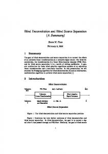
Table 1. Different microphone con¿gurations tested in the experiments. Con¿g Microphone Placement

3. EXPERIMENTAL SETUP FOR RECORDINGS

M1

We carried out our experiments in a room of dimensions 12ft by 9ft 11in by 8ft 2in. Two omni-directional microphones were mounted on the cell phone. One microphone, that served as the primary microphone of the the cell phone, was placed at the bottom front center of the cell-phone, which is the typical location of the microphone on a cell phone. The secondary microphone was placed at different locations along the back and side of the cell phone. We tested ¿ve realistic microphone con¿gurations listed in Table 1. The cellphone user was simulated by placing a loudspeaker near the primary microphone whereas the interfering source was placed at different locations in the room. Experiments with diffused noise were carried out in a slightly bigger room of dimensions 10ft 2in by 12ft 3in by 10ft. The diffused noise was simulated by placing an interfering loudspeaker in the corner of the room facing the walls. Speech was played on the primary speaker and noise or speech from an interfering speaker was played on the secondary speaker. These signals were recorded by the two microphones and the data was captured using an acquisition board and stored on a PC where it was processed. Nine different test cases were considered with different combinations of the primary speaker and the interference. These cases are listed in Table 2. The location of the primary speaker was ¿xed whereas the interfering source was placed at different locations in each of the test case. In Cases S5–S7 the primary speech was characterized by pauses in the conversation.

M2

4. PERFORMANCE ASSESSMENT Signal-to-interference ratio (SIR) is the conventional measure to assess the performance of BSS [2]. However, the computation of SIR requires a priori knowledge of the mixing as well as the unmixing ¿lters to determine the signal and interference contributions. In a real recording environment the mixing ¿lters cannot be measured, hence we can not rely on SIR for performance evaluation. Instead, we used a simple SNR measure to evaluate the performance of the algorithm. We calculated the SNR before BSS processing and subtracted it from the SNR after BSS processing to obtain performance improvement. The SNR was calculated by determining the noise energy in the silence periods of the speech. The exact location of these silence intervals was determined by the clean speech that was played on the primary loudspeaker. Note that such an information is not available in practice and is used here only for the sake of performance evaluation. 5. IMPACT OF MICROPHONE POSITIONS ON SPEECH SEPARATION In general, better noise suppression is obtained if microphones are spaced far apart. However, in cell phones, only a limited space is available for the placement of the secondary microphone. Initially, we evaluated the BSS performance using ¿ve microphone con¿gurations in the seven test cases S1–S7 listed in Table 2. We used unmixing ¿lter length of P = 128 in our experiments. We eliminated Microphone Con¿guration M4 earlier in our investigation for further consideration because of its relative poor performance in the ¿rst seven test cases of Table 2. For the four remaining microphone

1635

M3 M4

M5

Test Case S1 S2 S3 S4 S5 S6 S7 S8 S9

Table 2. Test cases used in the experiments. Primary Speaker Secondary/Interfering Noise Female Speech Female Train Female Pub Male Car Male and Female Train station with pauses Female with pauses Pub Male with pauses Train Female Diffused pub noise Female Diffused pub noise and male speaker

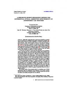
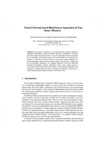
con¿gurations, we made recordings at ¿ve different primary input SNR levels of 15 dB, 10 dB, 5 dB, 0 dB, and < 0 dB. The results for the Test Cases S6 and S7 are shown in Fig. 1 and Fig. 2 respectively. From both the ¿gures it is clear that Microphone Con¿guration M1 results in an overall best performance over a range of input SNR values. We also note that the SNR gain improves at low input SNR, which is highly desired in cell-phone applications. We also evaluated the noise suppression performance using different unmixing ¿lter lengths. Fig. 3 shows the performance of the BSS algorithm for three different ¿lter lengths of 64, 128, and 256 using Microphone Con¿guration M1. We note that for high input SNR, the output SNR is somewhat the same for the three ¿lter lengths. More interestingly, for low input SNR, the performance improves with increasing ¿lter length. The processing complexity, however, increases with the ¿lter length as well. In an attempt to ease this complexity-performance trade-off, we suggest to use the length of P = 128. 6. POST-BSS PROCESSING Next, we evaluated the performance of BSS in the presence of diffused noise. The diffused noise was generated according to the setup described in Section 3. Our initial results showed that the diffused noise suppression was not up to the level reported in Section 5. In fact, it has been shown in [5] that, in the presence of diffused noise, the BSS separates the primary (desired) speaker from the secondary

Female In Pub Noise 16

12

10 8 6 4 2

10 8 6 4 2

0

0

í2

í2

í4 í5

0

5 10 15 20 SNR in the Primary Channel before processing

1 2 3 5

14

Improvement in SNR (dB)

12

Microphone Configuration

16

1 2 3 5

14

Improvement in SNR (dB)

Male In Train Noise

Microphone Configuration

í4 í5

25

0

5 10 15 20 SNR in the Primary Channel before processing

25

Fig. 1. SNR improvement versus input SNR for Test Case S6 using different microphone con¿gurations. Unmixing ¿lter length of P = 128 was used.

Fig. 2. SNR improvement versus input SNR for Test Case S7 using different microphone con¿gurations. Unmixing ¿lter length of P = 128 was used.

(noise) channel better than it can reject the diffused noise from the primary channel. The reason for this behavior is that the BSS steers a beam towards the desired speaker in the primary channel. While the speaker is captured in the separated output, part of the interference remains as the directivity pattern gain is not zero in the directions other than the direction of the speaker. On the other hand, the BSS steers a null towards the desired speaker in the secondary channel to recover the diffused noise arriving from all the directions other than the direction of the speaker. Since this separation is based on null steering, it does a better separation job than the primary channel [5]. Based on the above analysis we propose to utilize the noise output of the secondary channel to estimate the noise remaining in the output of the primary channel that also contains the desired speaker. The estimated noise is then subtracted from the primary channel output to further clean the desired speech signal. In frequency domain, the magnitude spectrum of the post-BSS processed speech is given by

and 2 6 6 Px = 6 6 4

3 7 7 7, 7 5

(9) where (·)T denotes transpose and Pyn (k) denotes the kth frequency bin of magnitude spectrum of the secondary BSS output for the nth frame of data. Note that the matrix Py consists of diagonal matrices stacked on top of each other. It’s pseudo inverse can be simpli¿ed as 2 N−1 P 1 6 i=0 Py2n−i (0) 6 6 6 0 6 † Py = 6 6 6 0 6 4 0

Ps = Px − Py h, (6) where Px is the magnitude spectrum of the primary channel output, Py is the magnitude spectrum of the secondary channel output and h is the transform vector of length L that maps the noise spectrum of the secondary BSS output to the noise spectrum output of the primary channel. We estimate h during the silence intervals using least squares and apply it during the speech duration. A voice activity detector is used to determine the silence periods in speech. A least-squares solution to h can be obtained as follows h = P†y Px ,

[Pxn (0) Pxn (1) . . . Pxn (L − 1)]T ˜T Pxn−1 (0) Pxn−1 (1) . . . Pxn−1 (L − 1) .. . ˜T ˆ Pxn−N +1 (0) Pxn−N +1 (1) . . . Pxn−N +1 (L − 1) ˆ

0 N−1 P i=0

Py2

1

n−i

(1)

3

...

0

...

0

0

..

0

...

.

0

N−1 P i=0

Py2

1 (L−1)

n−i

(10) The noise suppressed speech spectrum is constructed by using the magnitude spectrum obtained in (6) and the phase of the primary channel spectrum unaltered. The inverse FFT is then taken to obtain the noise suppressed speech.

(7)

where (·)† denotes pseudo inverse, and Py and Px contains the magnitude spectrum data collected from N silent frames and arranged as 3 2 diag ˆ [Pyn (0) Pyn (1) . . . Pyn (L − 1)] ˜ 7 6 diag Pyn−1 (0) Pyn−1 (1) . . . Pyn−1 (L − 1) 7 6 Py = 6 7 .. 5 4 . ˜ ˆ diag Pyn−N +1 (0) Pyn−N +1 (1) . . . Pyn−N +1 (L − 1) (8)

7. RESULTS OF POST-BSS PROCESSING We evaluated the post-processing module on the Test Cases S8 and S9 in Table 2. We used N = 3 and L = 1024 in our experiments. The SNR before BSS, after BSS, and after the post processing are listed in Table 3. As we note, the SNR gains at the output of BSS are signi¿cantly lower than the gains that were obtained earlier in the case of non-diffused noise. However, the use of post processing boosts up the gain to 9.8 dB and 8.7 dB for the Test Cases S8 and S9 respectively.

1636

7 7 7 7 7 7. 7 7 7 5

Female In Pub Noise for Mic Configuration 1 Filter Length

16

64 128 256

14

0 í0.5 0

12 Improvement in SNR (dB)

(a) Speech Mixture obtained from Primary Microphone 0.5

10

10

20 30 40 Time (b) Primary output after BSS

50

0.5 0

8 6

í0.5 0

4

0.5

10

20 30 40 Time (c) Primary Output after PostíProcessing

50

0

2

í0.5 0

0

10

20

30 Time

40

50

í2 í4 í5

0

5 10 15 20 SNR in the Primary Channel before processing

25

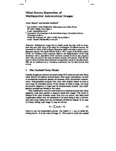
Fig. 4. Time-domain plots of the primary mixture, primary BSS output, and primary post-BSS processed outputs. Test Case S8 was used.

Fig. 3. SNR improvement versus input SNR for Test Case S6 using different unmixing ¿lter lengths P . Microphone Con¿guration M1 was used. Table 3. Results of the post-BSS processing in diffused noise case for Microphone Con¿guration M1. Unmixing ¿lter length of P = 128 was used. Test SNR SNR Post-Proc. SNR Case Before BSS After BSS SNR Improvement (dB) (dB) (dB) (dB) S8 1.8 6.6 11.6 9.8 S9 2.4 6.5 11.1 8.7

For the Test Case S8, the time domain plots of the mixture obtained from the primary microphone, the separated primary signal obtained after BSS, and the noise suppressed signal obtained after the post processing are shown in Fig. 4. The corresponding spectrograms are shown in Fig. 5 for a small segment of the speech sample.

Fig. 5. Spectrogram plots of the primary mixture, primary BSS output, and primary post-BSS processed outputs. Test Case S8 was used. 9. REFERENCES

8. CONCLUSIONS

[1] P. C. Loizou, Speech Enhancement: Theory and Practice, CRC, 2007.

We demonstrated the feasibility of employing multiple microphones on a cell phone to suppress unwanted interference in the uplink speech of the user. In the case of point interferences we were able to obtain 10–15 dB of SNR improvement when the input SNR is close to 0 dB. For diffused noise, we proposed the use of a post-BSS processing stage to further enhance the BSS speech output resulting in an overall SNR gain of about 8–9 dB. The recordings for all the experiments were made in a real acoustic environment using two microphones on a cell phone. Different locations of the secondary microphone were analyzed and an optimal location was suggested at the back of the cell phone. The BSS algorithm was also optimized so that the processing could ¿t the architecture of a low-power audio codec for real-time processing. The impact of unmixing ¿lter length on the interference-rejection performance was also studied and it was concluded that a ¿lter length of 128 provides the best trade-off between complexity and performance.

[2] L. Parra and C. Spence, “Convolutive blind separation of nonstationary sources,” IEEE Trans. Speech and Audio Processing, vol. 8, pp. 320–327, May 2000.

1637

[3] E. Visser and T.-W. Lee, “Blind source separation in mobile environments using a priori knowledge,” IEEE Int. Conf. Acoustics, Speech, Signal Processing, pp. 893–896, 2004. [4] S. Haykin, Unsupervised Adaptive Filtering, Volume 1: Blind Source Separation, John Wiley & Sons, Inc., 2000. [5] Y. Takahashi, T. Takatani, K. Osako, H. Saruwatari, and K. Shikano, “Blind spatial subtraction array for speech enhancement in noisy environment,” IEEE Trans. Audio, Speech and Language Processing, vol. 17, pp. 650–664, May 2009.