exist many adaptive network solutions (representations), which succeed in recovering the original signals even in the absence of precise identifiability [5,6].
Blind Source Recovery: Some Implementation and Performance Issues Khurram Waheed and Fathi M. Salam Circuits, Systems, And Neural Networks Laboratory Department of Electrical and Computer Engineering Michigan State University East Lansing, MI 48824-1226 Abstract This paper discusses the implementation of our proposed algorithms for Blind source Recovery based on constrained optimization using the state-space framework. Two simulation examples are presented where the mixing environment is modeled as FIR and IIR, respectively. The rate of convergence using the proposed implementation for these particular environment models is compared for various classes of data. Conclusions are derived for effectiveness of these techniques in various practical problems.
1: Introduction Blind Source Recovery (BSR), or Multi-channel Blind Deconvolution (MCBD), is a more practical problem formulation that combines Blind Source Separation and Blind Source Deconvolution. We postulate state space models for both the mixing environment and demixing (i.e. recovering) adaptive network. Blind Source Recovery (BSR) has currently been a very active research area in the arena of adaptive signal processing and autonomous learning. The BSR problem denotes recovering original sources from environments that may include convolution, transients, and even possible nonlinearity. BSR has several potential application domains including e.g., wireless telecommunication systems, sonar and radar systems, audio and acoustics, image enhancement and biomedical signal processing (EEG/MEG, EOG, EMG, ECG signals). Our proposed recent algorithms for blind source recovery have been derived based on multi-variable state space constrained optimization and the calculus of variations, which guarantee, global and analytical, optimal results. It can be further demonstrated that other derivations for similar algorithms give good results only when they are inline with this proposed generalized optimization procedure [2,3,4,6]. The state space notion provides a compact representation, which is capable of handling both time delayed and filtered versions of signals in an organized manner [1,3,5,6]. Unlike the transfer function models, the state-space provides an efficient internal description of a system. Moreover, there are various possible equivalent state space realizations for a
system, and thus recovery of original sources can be achieved independent from (and even in the absence of) environment identifiability, i.e. determining the exact (or a specific function of) parameters of the environment. There exist many adaptive network solutions (representations), which succeed in recovering the original signals even in the absence of precise identifiability [5,6]. The existence of solutions that enable the recovery of original sources have been expressed as recoverability [1,3,5]. The state space model enables much more general description than standard finite/infinite impulse response (FIR/IIR) convolutive filtering. All known filtering (dynamic) models, like AR, MA, ARMA, ARMAX and Gamma filtering can be considered as special cases of the more general state space representation. Existence and constructions of a theoretical solution to the Blind Source Recovery problem can be easily derived using the state space, given a structure of the environment. The inverse for a state space representation is easily derived subject to the invertibility of the instantaneous relational mixing matrix between input-output − in case this matrix is not square; the condition reduces to the existence of pseudoinverse of this matrix.
2: Blind Source Recovery: Problem Taxonomy In the most general setting, the mixing/convolving environment may be represented by an unknown dynamic process/filter H with inputs being the independent sources s and the outputs being the measurements m. In this case, no structure is assumed about the model of the environment except that it is dynamic with fixed unknown parameters.
Unknown
s1 (t ) s2 (t )
sn (t )
Mixing/Convolving Network/Filter
H
m1 (t ) m2 (t )
mm (t )
Demixing/Deconvolving Network/Filter
H
Figure 1: General Blind Source Recovery Framework
y1 (t ) y2 (t )
yN (t )
The processing network H must be constructed with the capability to compute the “inverse” (or the “closest to an inverse”) of the environment model. It is possible that an augmented network be constructed so that the inverse of the environment is merely a subsystem of the network with learning.
k
λk = Ak λk + Ck T
T
∂L
(2.6)
∂yk
∆A = −ηλk +1 X k
(2.7)
∆B = −ηλk +1 mk
(2.8)
T
T
(
T
T
)
2.1: Blind Source Recovery: Linear State-Space Formulation
∆ C = η ( I − ϕ ( y k ) y k ) C − ϕ ( yk ) X k
In the linear dynamic case, the environment model is assumed to be of the state space form X e (k + 1) = Ae X e (k ) + Be s(k ) (2.1)
The above derived update laws form a comprehensive algorithm and provides the update laws for the states, the co-states and all the parametric matrices in the state space. Note, that the states Xk are computed forward in time, while the co-states λk are computed backwards in time. The invertibility of the state space is guaranteed if the matrix D is invertible (or at least pseudo-invertible). In the above derived laws η - learning rate of the algorithm
m ( k ) = Ce X e ( k ) + De s ( k )
(2.2)
De s(k)
Be
+
Xe(k+1)
z-1I
Xe(k)
Ce
+
m(k)
Ae
Figure 2: State Space Separating Framework
In this case, the feedforward separating network will attain the state space form X ( k + 1) = A X ( k ) + B m ( k ) (2.3) y ( k ) = C X ( k ) + D m( k ) (2.4) D
m(k)
B
+
X(k+1)
z-1I
X(k)
C
+
y(k)
A
Figure 3: Linear Dynamic Environment Model
The existence of explicit solutions in this case has been shown in Salam et. al. [5, and the references therein]. This existence of solution ensures that the network has the capacity to compensate for the environment and consequently recover the original signals. Recoverability can thus be ensured. For the linear state-space the update laws have been derived in [5,6] as X k +1 = A X k + B mk (2.5)
∆D = η ( I − ϕ ( yk ) ykT ) D
(2.9) (2.10)
ϕ ( y ) - represents an element wise nonlinearity acting individually on each component of the output vector y, where the optimal non-linearity depends on the stochastic distribution of sources to be separated ∂p( y ) ∂y ϕ ( y) = − (2.11) p( y ) The update laws for the natural gradient update derived in [2,3] are in exact agreement with the update laws (2.9) and (2.10). The update law provided above becomes non-causal for the case of MIMO filtering structures, but practically can be easily implemented using standard time delay and buffer memory storage. A small latency in the recovered signal is acceptable for the BSR problem as long as the sample delay is fixed for all the recovered signals.
3: Simulation Examples We present two simulation results. One for the FIR type mixing environment and the other for IIR type mixing environment. The environment models for both systems were represented using MIMO canonical state space forms [5,6]. The demixing system is also formulated as a statespace network. For both the presented simulations, the demixing network is trained to be a two-sided (doubly finite) FIR filter i.e, the structure for matrices A and B is fixed and only matrices C and D are adaptively updated. The physical implementation is achieved using time-delayed configuration where the delay is equal to half the number of taps in the demixing filter. This formulation is chosen because of the inherent stability of an FIR structure. The proposed implementation is capable of even handling environments where the demixing system will be unstable
because of the presence of non-minimum phase zeros in the mixing environment. The convergence performance of the algorithm is measured using the multi-channel intersymbol interference benchmark, which is defined as [3] N
ISI k = ∑
∑∑ j
p
max p , j G pij
i =1
N
∑ j =1
G pij − max p , j G pij
∑∑ i
+ (3.1)
G pij − max p ,i G pij p
The algorithm is applied to the gamma, uniform, bimodal distributed sources and some combinations of the above. The algorithm converges in all cases with the worst ISI of – 23 dB in the case of uniform distributed sources. The algorithms work blindly without any assumption about the distribution structure of the sources. The convergence speed is still comparable to the cases where an optimal nonlinearity, for a given distribution structure of the sources, is chosen from start rendering the problem to be semi-blind. Environment Filter Taps
max p ,i G pij
1
where G(z) – Global Transfer Function G( z) = H ( z) * H ( z) (3.2) and H ( z ) = [ Ae , Be , Ce , De ] –Transfer Function of Environment H ( z ) = [ A, B, C , D] –Transfer Function of Network,
0.5
0.5
Estimated Inverse Filter Taps 2
1
0.5
0
0
0
0
-1
0
1
0.5
2 W11
-0.5
3
1
1.5
2 W12
-0.5
3
1
0.5
0
1
0
-0.5
0.5
-0.5
-1
0
-1
2 W13
-1
3
40
-0.5
0
20 w12
2
40
1
1
2 W21
3
1
1
0.5
2 W22
3
1
1
2 W23
3
0
1
2 W31
-0.5
3
0
20 w21
40
2 W32
Initial Global Transfer Function 1 0.5
0
20 w22
40
-0.5
2 W33
-0.2
3
0
20 w31
40
-1
0.5
20 iG11
40
-0.5 1.5
0
20 iG12
40
20 w32
40
-1
-0.5
1
20 iG21
0
40
20 iG13
-0.1
40
0
0.1
20 G11
40
1
0.5
20 iG22
40
-0.05
0
20 G12
40
-1
20 G22
40
20 iG23
1
0
0
20 iG31
40
-0.5
-0.1
40
20 iG32
40
-1
20 G32
40
20 G21
40
20 G31
40
0
0.05
-0.1
0
20 G23
40
0
20 G33
40
0.05
0
20 iG33
-1
40
0
-0.05
0
0
-0.05
Final Global Filter Multichannel Blind Source Separation 6 ISI for y1
4 ISI for y1
4
2
2
0
0.2
0.4
0.6
0.8 1 1.2 number of iterations
1.4
1.6
1.8
0 0
2 4
x 10
1
2
3
3 4 5 number of iterations
6
3 4 5 number of iterations
6
3 4 5 number of iterations
6
7
8 4
x 10
ISI for y2
3
2
ISI for y2
2
1
1
0
0.2
0.4
0.6
1.4
1.6
1.8
0 0 3
2 4
x 10
1
2
7
8 4
x 10
ISI for y3
0.8 1 1.2 number of iterations
2
ISI for y3
1
1 0
-1
0
0
Multichannel Blind Source Separation
0
40
1
Initial Global Filter
0
20 G13
0
0
2
-0.5 0
0
0.1
0
0
0 0 -0.5
-1
1
0.5
0.5
40
2
2
-0.5
0
20 w33
0
0
0
0.5
0
0
0
0 -0.5
-1
1
0.5
1
40
Estimated Inverse Filter
0
0
20 w23
0
0
Global Transfer Function 0.1 0.05
1
0
0
0
0
1
0 0
-0.5
1
0.5 0.5
40
2
0
-1
3
-1 0.5
-0.5 1
20 w13
0
0.2
0 0 -0.5
0
0 -2
0.5
0.5
-2 0.5
1
2
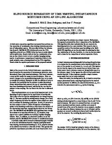
This simulation presents the results for 3 x 3 FIR filtering environment.
20 w11
0
3
0
0.2
0.4
0.6
0.8 1 1.2 number of iterations
1.4
1.6
1.8
0 0
2
1
2
4
x 10
Sub-Gaussian Data (Bi-modal)
7
8
Super Gaussian Data Multichannel Blind Source Separation
i =0
3
ISI for y1
(3.4)
2 1 0
where
0
1
2
3
3 4 number of iterations
5
3 4 number of iterations
5
3 4 number of iterations
5
6
7 4
x 10
0.5 = 0.1 −0.2
0.2 0 −0.3
0.4 −0.1 (3.5) −0.1
The problem is setup in the state space framework [5,6]. The theoretical inverse of this FIR filter will be an IIR filter of dimension 6 or higher. As remarked earlier we set up the problem for a doubly finite FIR filter inverse with 31 taps.
1 0
0
1
2
3
6
7 4
x 10
2
ISI for y3
0.3 , B2 0.7
ISI for y2
2
0.6
1 0
0
1
2
6
4
x 10
4
n −1
m(k ) = ∑ Bi s(k − i ) + v(k ) 1.0 0.5 0.8 0.9 −0.3 B0 = −0.7 1.2 −1.0 , B1 = 0.4 1.0 0.9 1.0 −0.8 0.6 0.3 v(k ) - additive Gaussian noise
0
2
Mixing Filter
3.2: Simulation I
1
1
0
3.1: Choice of Nonlinearity As defined above in (2.11), the optimal nonlinearity for the update laws depends on the probability density function of the outputs, which upon convergence of algorithm is similar to the probability density of the independent sources. We have used an adaptive nonlinearity, which depends on the batch kurtosis of output of the demixing system. This nonlinearity converges to the optimal non-linearity for the demixing system as the network outputs approach stochastic independence. This nonlinearity, however, fails to give good results for sources with densities close to Gaussian. κ ( y ) ≥ 1 : super-gaussian ϕ ( y ) = y + κ 4 ( y ) tanh( β y ) where 4 κ 4 ( y ) ≤ −1: sub-gaussian (3.3) where κ 4 ( y ) - batch kurtosis of the output signals
1
0.5
7 4
x 10
Sub-Gaussian Data (Uniform)
Figure 4: Results for 3 x 3 FIR Filtering Environment
3.3: Simulation II
Multichannel Blind LMS 4
m −1
n −1
∑ A m( k − i ) = ∑ B s ( k − i ) + v ( k ) i
i =0
1.0
0.5 0.8 0.06 0.4 ,A = ,A = 1.0 0.8 −0.3 0.16 0.1
0
1
1
1
0.2 0.5
0.4 0
0.2
-0.5 -1
0
4
8 h11
12
-0.2
16
1
4
8 h12
12
-0.5
16
1.5
0
4
8 h21
12
-0.5
16
1
-0.5
0
4
8 h22
12
-1.5
16
0
20
40
20
40
60
-0.5
0
20
40
60
80
20
40 w22
60
80
0
-0.02
22
21
20
40
-0.02
60
20
40
60
80
0
20
40
60
80
0.6
-0.01
0
0
0.8
0
G(z)
22
F(z) 0
0
-0.01
0.01
0.5 0
-1
0.4 0.2 0
0
20
Initial Global Filter
40
60
80
-0.2
Final Global Filter Multichannel Blind LMS
Multichannel Blind LMS
4
3 2.5
3 ISI for s1
2 1.5 1
2 1
0.5 0
1
2
3
4 5 number of iterations
6
7
8
0 0
9 4
1
2
3
x 10
4
3
3 ISI for s2
4
2
4 5 6 number of iterations
7
4 5 6 number of iterations
7
8
9 4
x 10
2 1
1
0
1
2
3
4 5 number of iterations
1
6
7
8
9 4
x 10
Sub-Gaussian Data (Bi-modal)
1
2
3
8
9 4
x 10
Sub-Gaussian Data (Uniform)
This paper presents the simulated results for both an FIR and an IIR mixing/filtering environment using our proposed algorithm for BSR. The problem is setup in a state-space framework and we have used an adaptive non-linearity dependent purely on the statistics of the network output. It is shown that the algorithm is able to converge for a variety of source distributions. It is also observed that the proposed algorithms can be implemented using usual memory buffered time delay for real-world applications. Restricting the demixing network to be a doubly finite impulse response filter, we observe that the algorithm is able to converge to this equivalent FIR network even when the intended/implied demixing IIR system is unstable.
80
0.01
0.2
0.02
1
0
60
0.02
0.4
-0.2
60
1.5
-0.5
ISI for s1
-1
80
G(z)
-0.5
60
0.5
ISI for s2
60
G(z)12
G(z)11
12
F(z)11
F(z) 40
1
0
40 w21
0 20
40 w12
Estimated Inverse Filter
0
-1
F(z)21
20
0.6
0
20
-0.5 0
0.8
0.5
0
0
Final Global Transfer Function 1
1
0
-0.6
80
0.5
Mixing Filter
-1.5
60
-1 0
7
9 4
x 10
1.5
Initial Global Transfer Function 2
-2
40 w11
0
0
-1
20
1
0.5
-0.5
0
0.5
1
0
4 5 6 number of iterations
8
5: References
-0.4 0
7
0 -0.2
0
0
0.5
-1.5
0.4
0.6
4 5 6 number of iterations
4: Conclusions
Estimated Inverse Filter Taps 0.8
0.5
3
Figure 5: Results for 2 x 2 IIR Filtering Environment
2
The theoretical inverse of this IIR mixing environment will also be an IIR filter of dimension 8 or higher. Also one of the poles of the intended demixing network is outside the unit circle, making it an unstable filter. However, the problem is setup for a doubly finite FIR inverse filter with 61 taps. The algorithm is applied with gamma, uniform, and bimodal distributed sources and it converges in all cases with the worst ISI around –18 dB in the case of uniform distributed data. Even for these simulations, the convergence speed is comparable to the convergence speed achieved using optimal non-linearity for known source distributions. Environment Filter Taps (FIR equivalent) 1
2
2
0 0
(3.7)
1
3
2
1.0 0.8 −0.5 0.5 −0.125 0.06 B = , B = −0.5 0.2 , B = −0.1 0.7 1.0 0 v( k ) - Additive Gaussian noise 0
0 0
ISI for s2
j =0
2 1
(3.6)
i
where 1.0 A = 1.0
ISI for s1
This simulation presents the results for an IIR filtering environment model
3
0 0
1
2
3
Super-Gaussian Data
8
9 4
x 10
[1] F. M Salam. “An adaptive network for blind separation of independent signals.” Proc. of Int’l Symp. on Circuits and Systems, 1: pp. 431-1434, May 1993. [2] S. Amari, S. Douglas, A. Cichocki, and H. Yang: “Multichannel blind deconvolution and equalization using the natural gradient.” in Proc. of IEEE Wkshp on Signal Processing: Adv. in Wireless Comm., pp. 101– 104, Paris, France, 1997. [3] L. Zhang and A. Cichocki: “Blind deconvolution of dynamical systems: A state space approach”, Journal of Signal Processing, Vol. 4, No. 2, Mar. 2000, pp. 111-130. [4] T. W. Lee, A. J. Bell, and R. Orglmeister, “Blind Source Separation of Real World Signals ", Proc. of IEEE Int’l Conf. on Neural Networks, June 1997, Houston, pp 2129-2135. [5] F. M. Salam and G. Erten; “The State Space Framework for Blind Dynamic Signal Extraction and Recovery”; Proc. of Int’l Symp. on Circuits and Systems, 1999, Volume: 5, 1999; pp. 66 –69 [6] F. M. Salam, G. Erten and K. Waheed: “Blind Source Recovery: Algorithms for Static and Dynamic Environments”; Int’l Joint Conf. on Neural Networks, Washington, D.C., July 2001.