Implementing the simplex method as a cutting-plane method Csaba I. F´abi´an∗†
Olga Papp∗†
Kriszti´an Eretnek†
Abstract We show that the simplex method can be interpreted as a cutting-plane method, assumed that a special pricing rule is used. This approach is motivated by the recent success of the cutting-plane method in the solution of special stochastic programming problems. We compare the classic Dantzig pricing rule and the rule that derives from the cutting-plane approach. We focus on the special linear programming problem of finding the largest ball that fits into a given polyhedron.
Keywords. Simplex method, cutting-plane method, linear programming, convex programming, stochastic programming.
1
Introduction
Due to their relative simplicity and practical effectiveness, simplex-type and cutting-plane methods have been intriguing researchers since the invention of these methods. The simplex method was developed by Dantzig in 1947 and published in 1951 [3]. It was the first effective method for the solution of linear programming problems, and to this day it is considered an effective practical method, the method of choice for many problem types. A practical state-of-art summary of simplex computational techniques with many experimental observations can be found in Maros’s book [22]. On the other hand, worst-case complexity of the simplex method is exponential, see [13]. The gap between practical effectiveness and theoretical complexity was bridged by Borgwardt [1] and Spielman and Teng [30]. Cutting-plane methods for convex problems were proposed by Kelley [12], and Cheney and Goldstein [2] in 1959-1960. These methods are considered fairly efficient for quite general problem classes. However, according to our knowledge, efficiency estimates only exist for the continuously differentiable, strictly convex case. An overview can be found in Dempster and Merkovsky [5], where a geometrically convergent version is also presented. In recent years, cutting-plane approaches proved remarkably effective for certain special stochastic programming problems; see [14] for problems with Integrated Chance Constraints, [16] for minimising Conditional Value at Risk, and [7], [28], [18] for problems involving Second-order Stochastic Dominance. Each of these stochastic programming problems can be formulated as linear programming problems having excessively many constraints. A cutting-plane method for the primal problem can be viewed as a special simplex method for the dual problem. In this paper we examine the special pricing rule that derives from the cutting-plane approach. In section 2 we consider a general linear programming problem, and the corresponding cutting-plane method that approximates the feasible polyhedron. In section 3 we consider the special linear programming problem of finding the largest ball that fits into a given polyhedron. This type of problem can be formulated as minimisation of a polyhedral convex function, and the corresponding cutting-plane method approximates this objective function. ∗ Institute † E¨ otv¨ os
of Informatics, Kecskem´ et College, 10 Izs´ aki u ´ t, 6000 Kecskem´ et, Hungary. E-mail:
[email protected]. Lor´ and University, Budapest, Hungary
1
A computational study is presented in section 4. We compare the classic Dantzig pricing rule and the cutting-plane pricing rule on general linear programming problems, and also on ball-fitting problems. The results show characteristic differences. Conclusions are drawn in section 5. Some of the proofs presented in sections 2 and 3 exploit the theoretical equivalence of the primal and dual simplex methods. To put this equivalence more precisely, a dual simplex method applied to the dual problem can be interpreted as a simplex method applied to the primal problem.
1.1
Notes on the equivalence of the primal and the dual simplex methods
The dual simplex method was developed by Lemke in 1954 [17]. According to our knowledge, the equivalence of the simplex method and the dual simplex method was first noticed by Pr´ekopa in the nineteen sixties [27], inspired by the essays [15]. Pr´ekopa presented the equivalence in his 1967 - 1969 linear programming courses at the E¨otv¨os Lor´and University of Budapest. This topic was later left out of the curriculum, but some of the students noticed the equivalence by themselves: Terlaky [31] in the nineteen seventies, and one of the authors of this paper in the nineteen eighties. Concerning written publications, Pr´ekopa [25] treated the simplex method and the dual simplex method in a unified form, as row and column transformations, respectively, on an appropriate square matrix. Equivalence of simplex and dual simplex steps is stated in Pr´ekopa [26] in the following form: primal transformation formulas result the same tableau that we obtain when we first carry out the dual transformation formulas and then take the negative transpose of the tableau. Padberg [24] observes the equivalence of the primal and the dual simplex methods with the remark that the numerical behaviour of the two methods may be very different. Vanderbei [33] states the equivalence in the following form: there is a negative transpose relationship between the primal and the dual problem, provided that the same set of pivots that were applied to the primal problem are also applied to the dual. In the appendix we also give a brief proof to the primal-dual equivalence. (We think the simplicity of this proof justifies its inclusion.) This proof is based on a special relationship between primal and dual bases. This relationship was also observed in former works: an asymmetric form is described in Kall and Mayer [11], and a symmetric form in [9].
1.2
Notation and clarification of terms
Let us consider the primal-dual pair of problems (1.P)
Ax ≤ b x≥0 max cT x,
(1.D)
AT y ≥ c y≥0 min bT y,
(1)
where A is an m × n matrix, and the vectors b and c have appropriate dimensions. We assume that both problems in (1) are feasible (and hence both have a finite optimum). We will solve these problems by the simplex and the dual simplex method, respectively. To this end, we formulate them with equality constraints, by introducing slack and surplus variables: (2.P)
Ax + Iu = b (x, u) ≥ 0 max cT x,
(2.D)
y T A − v T I = cT (y, v) ≥ 0 min y T b,
(2)
where I denotes identity matrix of appropriate dimension (m × m in the primal problem and n × n in the dual problem). Notation for the primal problem. A basis B of the primal problem is an appropriate subset of the columns of the matrix (A, I). A basis is said to be feasible if the corresponding basic solution is non-negative.
2
Let B denote the basis matrix corresponding to the basis B. Given a vector z ∈ IRn+m , let z B ∈ IRm denote the sub-vector containing the basic positions of z. Specifically, let (c, 0)B denote the basic part of the objective vector. Let y denote the shadow-price vector (a.k.a. dual vector) belonging to basis ¡ B. This is ¢ determined by the equation y T B = (c, 0)TB . The reduced-cost vector belonging to basis B is AT y − c, y ∈ IRn+m . Notation for µ the¶dual problem. A basis C of the dual problem is an appropriate subset of the rows of A the matrix . −I Let x denote the shadow-price vector belonging to basis C. This is determined by the equation Cx = (b, 0)C , where C is the basis matrix, and the right-hand side expression denotes the basic part of the vector (b, 0). The reduced-cost vector belonging to basis C is ( b − Ax, x ) ∈ IRm+n . Basis C is said to be dual feasible if the reduced-cost vector is non-negative. Applying the simplex method to the primal problem. We assume that a feasible starting basis is known, and use the phase-II simplex method. This is an iterative procedure that visits feasible bases. The method stops if the current reduced cost vector is non-negative. Otherwise a simplex step is performed: A column with a negative reduced cost is selected for entering the basis. The pivot element must be positive, and the selection of the outgoing column must guarantee the feasibility of the successive basis. We view the simplex method as a sequence of steps satisfying the above requirements. An implementation of the simplex method should of course uniquely determine the entering and the leaving column in each step. The technical jargon for the rule determining the entering column is pricing rule. In this paper we compare two pricing rules: the classic one that selects the column with the minimal (negative) reduced cost, and a new rule derived from the cutting-plane approach. Applying the dual simplex method to the dual problem. We assume that a dual feasible starting basis is known, and use the phase-II dual simplex method. This is an iterative procedure that visits dual feasible bases. The method stops if the current basic solution vector is non-negative. Otherwise a dual simplex step is performed: A negative component is selected in the current basic solution, and the corresponding basic column leaves the basis. The pivot element must be negative, and the selection of the incoming column must guarantee the dual feasibility of the successive basis. We view the dual simplex method as a sequence of steps satisfying the above requirements. An implementation of the dual simplex method should of course uniquely determine the leaving and the entering column in each step.
2
A cutting-plane method approximating the feasible domain
Let aj (j = 1, . . . , n) denote the columns of matrix A. Problem (1.D) can be written in the form ¯ © ª min bT y where Y := y ∈ IRm ¯ y ≥ 0, aTj y ≥ cj (j = 1, . . . , n) . y ∈Y
(3)
Let us solve problem (3) by the cutting-plane method. This is an iterative method that builds a model of the feasible domain in the form ¯ © ª YJ := y ∈ IRm ¯ y ≥ 0, aTj y ≥ cj (j ∈ J ) , (4) where J ⊆ {1, . . . , n} denotes the set of cuts found so far. The model problem min bT y y ∈YJ
3
(5)
is then solved and a new cut is added as needed. In this paper we assume that each occurring model problem has finite optimum. – This is achieved by a broad enough initial set of cuts as we assumed that the problem (1.D) has a finite optimum. Let us rehearse steps of the cutting-plane method as applied to the present problem: Algorithm 1 A cutting-plane method approximating the feasible polyhedron. 1.0 Initialise. Let J ⊂ {1, . . . , n} be such that the model problem (5) has a finite optimum. 1.1 Solve the model problem (5). Let y ? be an optimal solution. 1.2 Check. If y ? ∈ Y then stop. 1.3 Update the model problem. © ª Select deepest cut, i.e., j ? ∈ arg min aTj y ? − cj . 1≤j≤n
Let J := J ∪ {j ? }, and repeat from step 1.1. The model problem can be formulated as (6.D), below; a relaxation of (1.D). This is a linear programming problem that makes a primal-dual pair with (6.P). (6.P)
AJ xJ ≤ b xJ ≥ 0 max cTJ xJ ,
(6.D)
ATJ y ≥ cJ y≥0 min bT y,
(6)
where AJ denotes the sub-matrix of A containing the columns aj (j ∈ J ). Similarly, xJ and cJ denote respective sub-vectors of x and c, containing positions j ∈ J . According to our assumption, both problems in (6) have a finite optimum. Let us consider the series of model problems (6.D) occurring in the course of the cutting-plane process. Each successor problem in this series is obtained by adding a constraint to its predecessor. Having solved the predecessor problem by a simplex-type method, a dual feasible starting basis is easily constructed for the successor problem. Remark 2 Due to this warm-start potential, the dual simplex method is an effective and time-honoured means of solving the model problems in the cutting-plane process. Instead of solving the current model problem (6.D) by the dual simplex method, we can solve (6.P) by the simplex method. The following algorithm is a re-formulation of the previous one. Actually it is more specific in some points, like the handling of bases. We assume that a feasible basis is known for the primal problem (1.P). Algorithm 3 A re-formulation of algorithm 1. 3.0 Initialise. Let B ⊂ {1, . . . , n + m} be a feasible starting basis for the primal problem (1.P). Let J ⊂ {1, . . . , n} consist of the non-slack columns in B. 3.1 Solve the model problem (6.P) by the simplex method starting from basis B. Let B ? denote the optimal basis, and y ? the corresponding shadow-price vector. 3.2 Check. If aTj y ? ≥ cj holds for 1 ≤ j ≤ n, then stop. 4
3.3 Update the model problem. © ª Select j ? ∈ arg min aTj y ? − cj . 1≤j≤n
Let J := J ∪ {j ? }, B := B ? , and repeat from step 3.1. Observation 4 Algorithm 3 can be interpreted as solving problem (1.P) by the simplex method. Indeed, B? is a feasible basis for problem (1.P). Step 3.2 performs the regular optimality check on the columns of the matrix A. Slack columns need not be checked because they are included in the model problem. Step 3.3 selects a column having minimal (negative) reduced cost. This is the classic simplex pricing rule. (Having moved to step 3.1 from step 3.3, clearly j ? will be the first column entering the basis in course of solving the model problem.) The above classic simplex pricing rule is also called Dantzig pricing rule, after the seminal book [4]. Assume that in the simplex method of step 3.1, the classic pricing rule is used: the column having minimal reduced cost enters the basis. This results a special pricing rule applied in the simplex method of algorithm 3: Definition 5 Cutting-plane pricing rule. At any stage of the method, let J ⊂ {1, . . . , n} denote the set of the indexes of those x variables that have already been basic. In the subsequent pricing pass, columns in J ∪ {n + 1, . . . , n + m} are preferred to columns in {1, . . . , n} \ J , as candidates for entering basis. If there are columns in the set J ∪ {n + 1, . . . , n + m} with negative reduced costs, then we select the one having minimal reduced cost. If each column in J ∪ {n + 1, . . . , n + m} has a non-negative reduced cost, then we consider the set {1, . . . , n} \ J . From the latter set we also select the column having minimal reduced cost. As mentioned in remark 2, the dual simplex method is traditionally used for the solution of the model problems in the cutting-plane process of algorithm 1. We now see that the whole cutting-plane process can be implemented as a single dual simplex method. This follows from observation 4, and the general equivalence between the simplex method applied to the primal problem on the one hand, and the dual simplex method applied to the dual problem on the other hand.
3
A cutting-plane method approximating the objective function
In this section we deal with special problems of the form (7). For motivation, let us consider the primal-dual pair of problems (1), and suppose we want to find a ’central’ point in the feasible domain of problem (1.D). Constraints in (1.D) have the form aTj y ≥ cj (j = 1, . . . , n). Given a tolerance ζ > 0, a vector y satisfies the jth constraint with this tolerance if aTj y + ζ ≥ cj holds. We want to find a point y ≥ 0 that satisfies each constraint with minimum tolerance. This is described by the following problem: AT y + ζ1 ≥ c y ≥ 0, ζ ∈ IR min ζ,
(7)
where 1 = (1, . . . , 1)T denotes a vector of appropriate dimension. A negative tolerance means that the current solution satisfies a constraint set ’uniformly’ stricter than that of (1.D). – If (1.D) is feasible and the Euclidean of the ¯ © norms ª columns aj are each 1, then (7) finds a maximum-radius ball that fits into the polyhedron y ¯AT y ≥ c , such that the centre of the ball falls into the positive orthant. Problem (7) is always feasible as ζ may take positive values. To ensure a bounded objective, we add the constraint 1T y ≤ d where d is a (large) constant. For reasons of symmetry, we add this constraint in the form −1T y ≥ −d. We get (8.D) that makes a primal-dual pair with (8.P) :
(8.P)
Ax − ξ1 ≤ 0 1T x = 1 x ≥ 0, ξ ≥ 0 max cT x − dξ,
(8.D)
5
AT y + ζ1 ≥ c −1T y ≥ −d y ≥ 0, ζ ∈ IR min ζ.
(8)
The above pair of problems are similar to those treated by Dantzig’s self-dual parametric simplex method described in [4]. But the solution method we propose is different; in our case, e.g., d is constant. Problem (8.D) can be formulated as minimisation of a polyhedral convex function over a simplex, formally ¯ © ª © ª min ϕ(y) where ϕ(y) := max cj − aTj y , U := y ∈ IRm ¯ y ≥ 0, 1T y ≤ d . (9) y ∈U 1≤j≤n Clearly (y ? , ζ ? ) is an optimal solution of problem (8.D) if and only if y ? is an optimal solution, and ζ ? is the optimal objective value, of problem (9). We solve problem (9) by a cutting-plane method that builds the model function ª © (10) ϕJ (y) := max cj − aTj y , j∈J
where J ⊆ {1, . . . , n} denotes the set of cuts found so far. Let us rehearse steps of the cutting-plane method as applied to the present problem: Algorithm 6 A cutting-plane method approximating the objective function. 6.0 Initialise. Let J ⊂ {1, . . . , n}, J 6= ∅. 6.1 Solve the model problem min ϕJ . U
Let y ? be an optimal solution. 6.2 Check. If ϕJ (y ? ) ≥ ϕ(y ? ) then stop. 6.3 Update the model function. Select j ? ∈ {1, . . . , n} such that l(y) = cj ? − aTj? y be a support function to ϕ(y) at y ? . Let J := J ∪ {j ? }, and repeat from step 6.1. The model problem in step 6.1 has an optimal solution since the feasible domain is bounded and the objective function is finite due to J 6= ∅. The criterion of step 6.2 clearly implies that y ? is an optimal solution of problem (9) because we have min ϕ ≥ min ϕJ = ϕJ (y ? ) ≥ ϕ(y ? ). U
U
The model problem can be formulated as (11.D), below; a relaxation of (8.D). This is a linear programming problem that makes a primal-dual pair with (11.P).
(11.P)
AJ xJ − ξ1 ≤ 0 1T x J = 1 xJ ≥ 0, ξ ≥ 0 max cTJ xJ − dξ,
(11.D)
ATJ y + ζ1 ≥ cJ −1T y ≥ −d y ≥ 0, ζ ∈ IR min ζ,
(11)
where the notation is the same as in the analogous case (6). Since (11.D) has an optimal solution, it follows from LP duality that (11.P) has an optimal solution. Clearly (y ? , ζ ? ) is an optimal solution of the dual problem (11.D) if and only if y ? is an optimal solution of the model problem minU ϕJ , and ζ ? is the optimal objective value. Like in the previous section, we will interpret the cutting-plane method as a simplex method. To this end, let us formulate the pair of problems (8) with equality constraints by introducing slack variables in the primal problem and surplus variables in the dual problem. In the primal problem we add m slack columns. Together with the ξ-column, that makes m + 1 artificial columns. Feasible bases for the primal problem are easily constructed; specifically, given a single x-column, one can select m out of the m + 1 artificial columns that make a feasible basis with the x-column. 6
Algorithm 7 A simplex interpretation of algorithm 6. 7.0 Initialise. Let B ⊂ {1, . . . , n + 1 + m} be a feasible basis for the primal problem (8.P). Let J ⊂ {1, . . . , n} consist of the x-columns belonging to B. 7.1 Solve the model problem (11.P) by the simplex method starting form basis B. Let B ? denote the optimal basis, and (y ? , ζ ? ) the corresponding dual vector. 7.2 Optimality check. If (y ? , ζ ? )T (aj , 1) ≥ cj (j = 1, . . . , n) then stop. 7.3 Pricing. © ª Let j ? ∈ arg min (y ? , ζ ? )T (aj , 1) − cj . 1≤j≤n
Let J := J ∪ {j ? }, B := B ? , and repeat from step 7.1. Algorithm 7 is clearly a specific version of algorithm 6. (In order to see the equivalence of the respective second and third steps, let us just substitute ζ ? for ϕJ (y ? ) in algorithm 6. ) Observation 8 Algorithm 7 describes a simplex method applied to problem (8.P). Specifically, the pricing in step 7.3 selects a column having minimal (negative) reduced cost. Assume that in the simplex method of step 7.1, the classic pricing rule is used: the column having minimal reduced cost enters the basis. This is the cutting-plane pricing rule (definition 5) as applied to problem (8.P): At any stage of the method, let J ⊂ {1, . . . , n} denote the set of the indexes of those x variables that have already been basic. In the subsequent pricing pass, columns in J ∪ {n + 1, . . . , n + 1 + m} are preferred to columns in {1, . . . , n} \ J , as candidates for entering basis. If there are columns in the set J ∪ {n + 1, . . . , n + 1 + m} with negative reduced costs, then we select the one having minimal reduced cost. If each column in J ∪ {n + 1, . . . , n + 1 + m} has a non-negative reduced cost, then we consider the set {1, . . . , n} \ J . From the latter set we also select the column having minimal reduced cost. Remark 9 Assume now that in the simplex method of step 7.1, we use the above cutting-plane pricing rule. This results a further pricing rule in the simplex method of algorithm 7. This further pricing rule can of course be applied in step 7.1 ... Summing up all these, we obtain a recursive structure with a respective precedence set at each level of the recursion. Corollary 10 The cutting-plane algorithm 6 can be implemented as a single dual simplex method applied to problem (8.D). Proof. According to observation 8, algorithm 6 can be implemented as a simplex method applied to problem (8.P). This in turn is equivalent to a dual simplex method applied to the dual problem (8.D). In the appendix we give a proof to this equivalence. To keep discussion simple, though, we consider pairs of problems having only inequality constraints, in the form of (1). It remains to be seen that the result is applicable to the present pair of problems (8). First we may assume that the system of inequalities AT y ≥ c, −1T y ≥ −d, y ≥ 0 has no feasible solution. This can be achieved by adding a large number γ to each component of the vector c in the pair of problems (8). The polyhedral problem (9) changes accordingly, the modified objective function being ϕ(y) + γ. Thus the cutting-plane sequence of algorithm 6 remains the same. The simplex step sequences for (8.P) also remain the same: Let us consider an arbitrary basis of problem (8.P), and let (y, ζ) denote the
7
corresponding dual vector. If we add the same number γ to each component of c, then the dual vector will change to (y, ζ + γ), hence the reduced cost components remain unchanged. Under the infeasibility assumption, the constraint ζ ≥ 0 is redundant in problem (12.D), below:
(12.P)
Ax − ξ1 ≤ 0 1T x ≤ 1 x ≥ 0, ξ ≥ 0 max cT x − dξ,
(12.D)
AT y + ζ1 ≥ c −1T y ≥ −d y ≥ 0, ζ ≥ 0 min ζ.
(12)
It means that there exists an optimal solution (x? , ξ ? ) of (12.P) such that 1T x? = 1 holds. Problems (8.P) and (12.P) differ only in the latter problem having an extra column (the slack column belonging to the constraint 1T x ≤ 1). Hence any series of simplex steps that solves (8.P) can also be considered as a series of simplex steps that solves (12.P). (The slack vector of the constraint 1T x ≤ 1 never enters basis in the course of such a series.) The pair of problems (12) has only inequality constraints, hence the discussion in the appendix is applicable: any series of simplex steps that solves (12.P) can be interpreted as a series of dual simplex steps that solves (12.D). Since the slack vector of the constraint 1T x ≤ 1 never enters basis in the course of our primal series, it follows that the variable ζ is always basic in the course of the corresponding dual series. Hence this dual series can be interpreted as a series of dual simplex steps that solves (8.D). u t
4
Computational study
We compared the classic Dantzig pricing rule and the cutting-plane pricing rule on general linear programming problems, and also on ball-fitting problems. (The latter type of special problems were discussed in section 3.)
4.1
Implementation issues
We implemented a basic but usable form of the simplex method: revised method with the product form of the inverse, and multiple pricing. (The implementation was part of the preparation of the Informatics Master’s thesis of the third author of this paper.) The optimality tolerance of 1e − 5 was used in the test runs. We can either use the classic Dantzig pricing, or the cutting-plane pricing. We implemented the latter in a form slightly different from that of definition 5: In our implementation, column indices of problem (8.P) are divided into three categories: The first category contains the index of the variable ξ and the indices of the slack variables. The second category contains the indices of those x variables that have already been basic. The third category contains the indexes of those x variables that have not yet been basic. We prefer first-category indexes to second-category ones, and second-category indexes to third-category ones. Given a category, indices falling into this category are ordered according to reduced costs. We did not implement the recursive pricing rule of remark 9. For our ball-fitting test problems, we do not expect any significant improvement from the recursive pricing over the cutting-plane pricing; because using the latter, it took only 2 pivot steps at the average to recover optimality in step 7.1 of the solution.
4.2
Test problems
We considered 59 test problems from the NETLIB collection (the smaller ones). These are listed in table 1. Given a NETLIB problem, we constructed a problem of the form (8.P) using only the matrix A and the objective vector c of the NETLIB problem. The constant d was always set so large that increasing d would not change the optimal basis of (8.P). Assumed each A-column has an Euclidean © ¯ norm ofª 1, the dual problem (8.D) can be interpreted as fitting the largest ball into the polyhedron y ¯AT y ≥ c , such that
8
© ¯ ª the centre of the inscribed ball falls into the simplex y ¯ y ≥ 0, 1T y ≤ d . Though we did not scale the columns, we dub the problem (8.P) the max-ball variant of the relevant NETLIB problem. Given a NETLIB problem, we also constructed a problem of the form (13.P), below, using only the matrix A and the objective vector c of the NETLIB problem.
(13.P)
Ax + ξ1 ≥ 0 1T x = 1 x ≥ 0, ξ ≥ 0 min cT x + dξ,
(13.D)
AT y + ζ1 ≤ c 1T y ≤ d y ≥ 0, ζ ∈ IR max ζ.
(13)
The constant d was set so large that increasing d would not change the optimal basis of (13.P). Assumed each A-column aj has an Euclidean norm of 1, the ©dual ¯ problem ª(13.D) can be interpreted as finding the smallest ball that intersects each of the half-spaces y ¯ aTj y ≤ cj (j = 1, . . . , n), such that the centre of © ¯ ª the ball falls into the simplex y ¯ y ≥ 0, 1T y ≤ d . Though we did not scale the columns, we dub the problem (13.P) the min-ball variant of the relevant NETLIB problem. The max-ball variants and the min-ball variants are special problems: each can be formulated as the minimisation of a convex objective over a simplex, as described in section 3. We compared the Dantzig pricing rule and the cutting-plane pricing rule on the general NETLIB problems, and also on the special ball-variants.
4.3
Comparison of pricing rules on general LP problems
We solved the 59 NETLIB problems by the simplex method, comparing the Dantzig pricing rule and the cutting-plane pricing rule as described in section 2. Our basic simplex implementation could solve 59 − 4 = 55 problems when the Dantzig pricing was used, and 59 − 8 = 51 problems when cutting-plane pricing was used. Out of the 59 test problems, 50 could be solved by both pricing rules. On average, solving a problem using the cutting-plane pricing took twice as long as it did when using the Dantzig pricing. The ratio between iteration counts was similar. (Our implementation is not a state-of-art solver, but the quality of the implementation is the same for the two pricing rules.) Summing up, the cutting-plane pricing rule proved very much inferior to the Dantzig pricing rule on general problems.
4.4
Comparison of pricing rules on ball-variant problems
We solved the 118 ball-variant problems by the simplex method, comparing the Dantzig pricing rule and the cutting-plane pricing rule as described in section 3. Our simplex implementation could solve 118 − 7 = 111 problems when the Dantzig pricing was used, and 118 − 2 = 116 problems when cutting-plane pricing was used. Out of the 118 test problems, 110 could be solved by both pricing rules. The total run times for these 110 problems were: 409,453 seconds for the classic pricing, and 373,209 seconds for the cutting-plane pricing. Iteration counts and run times are listed in tables 2 - 3. We also constructed the performance profiles of our implementations. This measurement tool was introduced by Dolan and Mor´e (2002). As in the present paper we only have two methods to compare, we present the construction of performance profiles in a simplified form: Let P denote the set of problems, and let tp and t0p denote the times of solving problem p ∈ P with the classic simplex pricing and the cutting-plane pricing, respectively. We define performance ratios rp =
tp min{tp , t0p }
and
rp0 =
t0p min{tp , t0p }
(p ∈ P).
If a method failed to solve a problem, then we set the corresponding value to ∞. Let us consider r and r0 as random variables with equally probable outcomes rp and rp0 (p ∈ P), respectively. The corresponding 9
cumulative distribution functions are ρ(τ ) =
|{ p ∈ P | rp ≤ τ }| |P|
and
ρ0 (τ ) =
|{ p ∈ P | rp0 ≤ τ }| |P|
(τ ∈ IR).
The performance profiles are the graphs of these cumulative distribution functions. A profile nearer the top left corner indicates a better algorithm. The performance profiles of the classic (Dantzig) and the cutting-plane pricing rules are presented in figure 4. On the ball-variant problems, the cutting-plane pricing rule performs slightly better than the classic rule.
4.5
Comparison of the difficulty of general LP problems and their max-ball variant problems
In this test we compared the difficulty of solving a general linear programming problem, i.e., optimising a linear function over a polyhedron on the one hand; and of finding a central point in the same polyhedron on the other hand. – Namely, the problems compared are of the forms (1.D) and (8.D), but we constructed and solved the primal pairs. Given a NETLIB problem, we constructed a problem of the form (1.P) using only the matrix A and the vectors b, c of the NETLIB problem. We refer to the resulting problem as canonical problem in this comparison. For each of our 59 NETLIB problems, we solved both the canonical problem and the max-ball variant problem using the cutting-plane pricing rule. On average, the max-ball problems were solved in 85% less iterations than the canonical problems. (I.e., the ratio of iteration counts was about 1 : 6.) Considering running times, the max-ball problems were solved in half the time as the canonical problems. (The difference between the ratios of iteration counts and of solution times is due to longer iteration times in the ball-variant problems. This is the consequence of faster non-zero build up in our inverse representation. – We maintain a product-form inverse in our implementation. A more sophisticated inverse representation would of course mitigate nonzero build-up.) To sum up our results, finding a central point in a polyhedron seems significantly easier than optimising a linear function over the same polyhedron. This observation is in accord with our former working experience: The simplex method is very flexible in handling feasibility issues, and this flexibility is exploited in finding a central point.
5
Conclusion and discussion
In this paper we showed that the simplex method can be interpreted as a convex cutting-plane method, assumed that a special pricing rule is used in the simplex implementation. The cutting-plane pricing rule proved very much inferior to the classic Dantzig rule when compared on general LP problems. On the other hand, the cutting-plane rule proved slightly better than the Dantzig rule when tried on special LP problems that can be formulated as minimisation of a convex objective over a simplex. A variety of simplex pricing rules have been developed in the past decades; see Terlaky and Zhang [32] for a survey. In the successful simplex-based solvers, several pricing rules are implemented, and the solver employs the one that best fits the situation. Such a general pricing scheme was proposed by Maros [21]. We do not expect the cutting-plane pricing rule to be competitive with a sophisticated pricing scheme. On the other hand, we think that including the cutting-plane rule may be advantageous to a pricing scheme.
5.1
On the utility of finding the largest inscribed ball
When applying the plain cutting-plane approach to a constrained convex program, the optimal solution of the current model problem is selected as the subsequent test point. E.g., in algorithm 1 (section 2), the 10
subsequent test point is y ? . A useful idea is finding a ’central’ point in the current polyhedral model of the feasible domain, and selecting this as the subsequent test point. Different centres were proposed and tried, the most widely used being the analytic centre. The Analytic Centre Cutting-Plane Method was introduced by Sonnevend [29], and further developed by Goffin, Haurie, and Vial [10]. This method proved effective for many problems. A recent development in this direction is described in [23]. Here an interior-point constraint-generation algorithm is presented for semi-infinite linear programming, with a successful application to a healthcare problem. Considering the ease of finding the largest inscribed ball (section 4.5), we think that the centre of this ball can also be used as the subsequent test point when solving a constrained convex problem by the cutting-plane method. Verification of this conjecture requires further experimentation. In case of linear problems, algorithm 1 (section 2) can be easily modified according to the above observation: Let the subsequent test point be the centre of the largest ball inscribed into the current model of the feasible domain. However, we expect this method to be effective only if the original problem has an excessively large number of constraints, and especially in case of semi-infinite programming problems.
5.2
Comments on the primal-dual equivalence
The following question is raised in [11]: given the equivalence of the simplex method and the dual simplex method, how to explain their very different numerical behaviour? The difference in basis sizes gives a partial explanation: if m >> n then the dual method handles the inverses of smaller matrices. However, this observation holds true only if traditional basis inversion routines are used: Maros [22] developed a special row basis technique that enables simplex implementations using a working basis of size min(n, m). (The row basis technique is related to the equivalence of the simplex and the dual simplex methods.) Using the basis correspondence described in the appendix, special inversion modules can be developed that handle even smaller working bases. We can store and keep updating the inverse of the sub-matrix S in figure 3. A product-form inverse of the variable-size S matrix is straightforward to implement. Such an inversion module was used in [8], without reference to the primal-dual equivalence. Application of this inversion routine resulted a substantial decrease in running time. (Though it should be mentioned that in the special problems handled in [8], even the sub-matrices S had a special structure that could be exploited.) Individual upper bounds of the variables are an important factor of the different behaviour of the simplex and the dual simplex method. The primal-dual equivalence does not extend to individual upper bounds, hence a method making use of such bounds does not have an equivalent counterpart. Such variants of the dual simplex method were recently proposed by Maros [19], [20], together with computational studies that demonstrate the effectiveness of the new variants. Another advantage of the dual simplex method is observed in [22]: Devex-type pricing requires little additional cost.
References [1] Borgwardt, K.H. (1980). The simplex method: a probabilistic analysis. Number 1 in Algorithms and Combinatorics. Springer-Verlag, New York. [2] Cheney, E.W. and A.A. Goldstein (1959). Newton’s method for convex programming and Tchebycheff approximation. Numeriche Mathematik 1, 253-268. [3] Dantzig, G.B. (1951). Maximization of a linear function of variables subject to linear inequalities. In: Activity Analysis of Production and Allocation, (T.C. Koopmans, editor). Wiley, New York, 339-347. [4] Dantzig, G.B. (1963). Linear Programming and Extensions. Princeton University Press, Princeton.
11
[5] Dempster, M.A.H. and R.R. Merkovsky (1995). A practical geometrically convergent cutting plane algorithm. SIAM Journal on Numerical Analysis 32, 631-644. ´ (2002). Benchmarking optimization software with performance profiles. [6] Dolan, E.D. and J.J. More Mathematical Programming 91, 201-213. ´ bia ´n, C.I., G. Mitra, and D. Roman. Processing Second-Order Stochastic Dominance mo[7] Fa dels using cutting-plane representations. Mathematical Programming, Ser. A DOI 10.1007/s10107009-0326-1. ´ bia ´n, C.I., A. Pre ´kopa, and O. Ruf-Fiedler (2002). On a dual method for a specially struc[8] Fa tured linear programming problem. Optimization Methods and Software 17, 445-492. ´ bia ´n, C.I. and Szo ˝ ke, Z. (2007). Solving two-stage stochastic programming problems with level [9] Fa decomposition. Computational Management Science 4, 313-353. [10] Goffin, J.-L., A. Haurie, and J.-P. Vial (1992). Decomposition and nondifferentiable optimization with the projective algorithm. Management Science 38, 284-302. [11] Kall, P. and J. Mayer (2005). Stochastic Linear Programming. Models, Theory, and Computation. International Series in Operations Research & Management Science. Springer. [12] Kelley, J.E. (1960). The cutting-plane method for solving convex programs. Journal of the Society for Industrial and Applied Mathematics 8, 703-712. [13] Klee, V. and G.J. Minty (1972). How good is the simplex algorithm? In: Inequalities III. (O. Shisha, editor). Academic Press, 159-175. [14] Klein Haneveld, W.K. and M.H. van der Vlerk (2006). Integrated chance constraints: reduced forms and an algorithm. Computational Management Science 3, 245-269. [15] Linear Inequalities and Related Systems. (H.W. Kuhn and A.W. Tucker, editors.) Princeton University Press, 1956. ¨ nzi-Bay, A. and J. Mayer (2006). Computational aspects of minimizing conditional value-at-risk. [16] Ku Computational Management Science 3, 3-27. [17] Lemke, C.E. (1954). The dual method of solving the linear programming problem. Naval Research Logistics Quarterly 1, 36-47. [18] Luedtke, J. (2008). New formulations for optimization under stochastic dominance constraints. SIAM Journal on Optimization 19, 1433-1450. [19] Maros, I. (2003). A generalized dual phase-2 simplex algorithm. European Journal of Operational Research 149, 1-16. [20] Maros, I. (2003). A piecewise linear dual phase-1 algorithm for the simplex method. Computational Optimization and Applications 26, 63-81. [21] Maros, I. (2003). A general pricing scheme for the simplex method. Annals of Operations Research 124, 193-203. [22] Maros, I. (2003). Computational Techniques of the Simplex Method. International Series in Operations Research & Management Science. Kluwer Academic Publishers, Boston. [23] Oskoorouchi, M.R., H.R. Ghaffari, T. Terlaky, and D.M. Aleman. An interior point constraint generation algorithm for semi-infinite optimization with healthcare application. Mathematics of Operations Research, to appear in 2011. 12
[24] Padberg, M. (1995). Linear optimization and extensions. Springer. ´kopa, A. (1968). Linear Programming (in Hungarian). Bolyai J´anos Mathematical Society, Bu[25] Pre dapest. ´kopa, A. (1992). A very short introduction to linear programming. RUTCOR Lecture Notes 2-92. [26] Pre ´kopa, A. (2011). Private communication. [27] Pre ´ ski (2008). Optimization problems with second order stochastic do[28] Rudolf, G. and A. Ruszczyn minance constraints: duality, compact formulations, and cut generation methods. SIAM Journal on Optimization 19, 1326-1343. [29] Sonnevend, G. (1988). New algorithms in convex programming based on a notion of ’centre’ (for systems of analytic inequalities) and on rational expectations. In: Trends in Mathematical Optimization: Proceedings of the 4th French-German Conference on Optimization (K.H. Hoffmann, J.-B. Hirriart-Urruty, C. Lemarchal, J. Zowe, editors). Volume 84, pp. 311-327 of the International Series of Numerical Mathematics. Birkh¨auser, Basel, Switzerland. [30] Spielman, D.A. and S.-H. Teng (2004). Smoothed analysis of algorithms: why the simplex algorithm usually takes polynomial time. Journal of the ACM 51, 385-463. [31] Terlaky, T. (2010). Private communication. [32] Terlaky, T. and S. Zhang (1993). Pivot rules for linear programming: a survey on recent theoretical developments. Annals of Operations Research 46, 203-233. [33] Vanderbei, R.J. (2001, 2008). Linear Programming. Foundations and Extensions. International Series in Operations Research & Management Science. Springer.
13
Appendix: a brief proof to the primal-dual equivalence We work on the pair of problems (2). The primal problem and a basis B are illustrated in figure 1, the basis matrix being denoted by B. The dual problem and a basis C are illustrated in figure 2, the basis matrix being denoted by C.
A one-to-one mapping between primal and dual bases Let µ : {1, . . . , n + m} → {1, . . . , m + n} be defined as m + ` if ` ≤ n, µ(`) = ` − n if n < `. µ maps columns of the primal problem to rows of the dual problem. Specifically, columns of matrix A are mapped to surplus rows, and slack columns are mapped to rows of matrix A. Given a subset B of the columns of the primal problem, we can construct a subset C of the rows of the dual problem according to the rule: Let µ(`) ∈ C if and only if ` 6∈ B.
(14)
In words: – a row of matrix A is selected into C if and only if the corresponding slack vector is not in B, – a surplus row is selected into C if and only if the corresponding column of A is not in B. Proposition 11 The above rule results a one-to-one mapping between primal and dual bases. Proof. The rule obviously results a one-to-one mapping between the collection of subsets B ⊂ {1, . . . , n + m}, |B| = m; and the collection of subsets C ⊂ {1, . . . , m + n}, |C| = n. It remains to be seen that C is a basis of the dual problem if and only if B is a basis of the primal problem. We illustrate this in figure 3 : matrix B consists of columns belonging to set B, and matrix C consists of rows belonging to set C. Let us consider the shaded square matrix S that is the ’intersection’ of B and C. Clearly B is invertible if and only if S is invertible. Similarly, C is invertible if and only if S is invertible. u t Observation 12 Assume that B and C are corresponding primal and dual bases (i.e., assigned to each other by the mapping of proposition 11). Let (x, u) denote the basic solution belonging to B. Then x is the shadow-price vector belonging to C, and (u, x) is the reduced-cost vector belonging to C. Let (y, v) denote the basic solution belonging to C. Then y is the shadow-price vector belonging to B, and (v, y) is the reduced-cost vector belonging to B. Corollary 13 Assume that B and C are corresponding primal and dual bases. C is a dual feasible basis of the dual problem if and only if B is a feasible basis of the primal problem.
Extended-sense simplex and dual simplex steps Characteristics of the simplex and the dual simplex steps were summed up in section 1.2. In this section we relax the sign restrictions on the pivot elements. Moreover, we show that in the absence of degeneracy, these restrictions are redundant.
14
Extended-sense simplex steps for the primal problem. Let B and B0 be feasible bases of the primal problem. Suppose B and B 0 are neighbouring bases, i.e., considering them as sets, their set-difference B0 \ B has a single element that we denote by `. (In words, ` is the index that enters basis in course of step B → B 0 .) Then B → B 0 is an extended-sense simplex step if and only if there is a negative component at position ` of the reduced-cost vector belonging to B. The difference between a regular simplex step and an extended-sense simplex step is that negative pivot elements are not excluded in the latter. We say that B → B 0 is a degenerate step if the same basic solution belongs to B and B 0 . If an extendedsense simplex step B → B 0 is not degenerate, then it is a regular simplex step, because pivoting on a negative element would obviously destroy feasibility. Extended-sense dual simplex steps for the dual problem. Let C and C 0 be dual feasible bases of the dual problem. Suppose C and C 0 are neighbouring bases, i.e., their set-difference C \ C 0 has a single element that we denote by k. (In words, k is the index that leaves basis in course of step C → C 0 .) Then C → C 0 is an extended-sense dual simplex step if and only if there is a negative component at position k of the basic solution belonging to C. The difference between a regular dual simplex step and an extended-sense dual simplex step is that positive pivot elements are not excluded in the latter. We say that C → C 0 is a dual degenerate step if the same reduced-cost vector belongs to C and C 0 . If an extended-sense dual simplex step C → C 0 is not dual degenerate, then it is a regular dual simplex step, because pivoting on a positive element would obviously destroy dual feasibility. Equivalence of extended-sense simplex and extended-sense dual simplex steps. Let (B, C) and (B 0 , C 0 ) be pairs of corresponding primal and dual bases. The mapping of proposition 11 obviously keeps neighbours, hence the primal bases B and B0 are neighbouring if and only if the dual bases C and C 0 are neighbouring. In the following discussion we assume that they are neighbouring. Corollary 13 takes care of feasibility issues: C is a dual feasible basis if and only if B is a feasible basis, and C 0 is a dual feasible basis if and only if B0 is a feasible basis. In what follows we assume that all these feasibility requirements are satisfied. Proposition 14 C → C 0 is an extended-sense dual simplex step if and only if B → B 0 is an extended-sense simplex step. Proof. Let ` denote the index that enters basis in course of step B → B 0 , and let k denote the index that leaves basis in course of step C → C 0 . According to rule (14), we have k = µ(`). Let (y, v) ∈ IRm+n denote the basic solution belonging to C. According to the second part of observation 12, the reduced-cost vector belonging to B is (v, y). From the properties of mapping µ, we obviously have (y, v)µ(`) = (v, y)` . From the above definitions, B → B 0 is an extended-sense simplex step if and only if (v, y)` < 0, and C → C 0 is an extended-sense dual simplex step if and only if (y, v)k < 0. u t
Equivalence of the simplex and the dual simplex method We are going to show that the simplex method applied to the primal problem on the one hand, and the dual simplex method applied to the dual problem on the other hand, are equivalent methods. If no degeneracy is present, then extended-sense simplex steps are regular simplex steps, and extended-sense dual simplex steps are regular dual simplex steps; hence the statement is a straight consequence of proposition 14. Let B → B 0 be an extended-sense simplex step, and let C → C 0 be the corresponding extended-sense dual simplex step. By the first part of observation 12, C → C 0 is dual degenerate if and only if B → B 0 is degenerate. Assume now that B → B 0 is a regular simplex step. Obviously there exists a perturbation of the righthand-side vector that makes B → B 0 non-degenerate, while retaining it a simplex step. This shows that C → C 0 is a regular dual simplex step. (If C → C 0 is known to be a regular dual simplex step, then a similar procedure can be applied to show that B → B 0 is a regular simplex step.) 15
Figure 1: Basis B in primal problem (2.P)
16
Figure 2: Basis C in dual problem (2.D)
17
Figure 3: Corresponding bases B and C
18
problem name ADLITTLE AFIRO AGG AGG2 AGG3 BANDM BEACONFD BLEND BNL1 BOEING1 BOEING2 BORE3D BRANDY CAPRI DEGEN2 E226 ETAMACRO FFFFF800 FINNIS FIT1D FIT2D FORPLAN GFRD-PNC GROW15 GROW22 GROW7 ISRAEL KB2 LOTFI PEROLD PILOT4 RECIPELP SC105 SC205 SC50A SC50B SCAGR25 SCAGR7 SCFXM1 SCFXM2 SCORPION SCRS8 SCTAP1 SCSD1 SCSD6 SEBA SHARE1B SHARE2B SHELL SHIP04L SHIP04S STAIR STANDATA STANDGUB STANDMPS STOCFOR1 TUFF VTP-BASE WOOD1P
rows 56 27 488 516 516 305 173 74 643 351 166 233 220 271 444 223 400 524 497 24 25 161 616 300 440 140 174 43 153 625 410 91 105 205 50 50 471 129 330 660 388 490 300 77 147 515 117 96 536 402 402 356 359 361 467 117 333 198 244
columns 97 32 163 302 302 472 262 83 1175 384 143 315 249 353 534 282 688 854 614 1026 10500 421 1092 645 946 301 142 41 308 1376 1000 180 103 203 48 48 500 140 457 914 358 1169 480 760 1350 1028 225 79 1775 2118 1458 467 1075 1184 1075 111 587 203 2594
Table 1: NETLIB test problems
19
problem name ADLITTLE AFIRO AGG AGG2 AGG3 BANDM BEACONFD BLEND BNL1 BOEING1 BOEING2 BORE3D BRANDY CAPRI DEGEN2 E226 ETAMACRO FFFFF800 FINNIS FIT1D FIT2D FORPLAN GFRD-PNC GROW15 GROW22 GROW7 ISRAEL KB2 LOTFI PEROLD PILOT4 RECIPELP SC105 SC205 SC50A SC50B SCAGR25 SCAGR7 SCFXM1 SCFXM2 SCORPION SCRS8 SCTAP1 SCSD1 SCSD6 SEBA SHARE1B SHARE2B SHELL SHIP04L SHIP04S STAIR STANDATA STANDGUB STANDMPS STOCFOR1 TUFF VTP-BASE WOOD1P
classic pricing rule iterations run time (millisec) 24 16 22 15 213 3625 426 7797 128 140 73 47 36 406 67 329 20 15 2 1 1 1 36 109 725 33828 202 875 4 15 167 4672 2 16 68 62 54 375 88 141 18 219 11 47 13 110 8 15 6 15 41 63 11 62 8377 13172 143 187 312 2438 71 46 64 31 23 156 3 1 5 15 7 93 13 62 48 297 196 1453 88 125 9 31 3 31 262 375 109 110 594 38281 58 578 32 218 126 1485 59 438 24 188 211 5766 74 93 136 1344 187 1782
cutting-plane pricing rule iterations run time (millisec) 41 15 23 15 219 2078 717 20843 1030 34766 13 15 102 78 30 359 70 344 22 31 5 15 1 1 10 16 1634 34953 467 2516 5 31 55 578 3 31 29 32 34 234 64 93 12 156 2 16 1 15 2 1 949 3829 9 1 36 31 87 2297 10 47 57 31 227 281 387 2922 62 31 64 46 23 141 6 1 2 16 7 93 1 1 46 281 150 1172 59 78 21 63 3 31 235 234 92 78 572 36844 28 250 65 578 93 453 8 31 8 31 8 47 59 62 120 985 2 1 1079 13406
Table 2: Max-ball variants test results
20
problem name ADLITTLE AFIRO AGG AGG2 AGG3 BANDM BEACONFD BLEND BNL1 BOEING1 BOEING2 BORE3D BRANDY CAPRI DEGEN2 E226 ETAMACRO FFFFF800 FINNIS FIT1D FIT2D FORPLAN GFRD-PNC GROW15 GROW22 GROW7 ISRAEL KB2 LOTFI PEROLD PILOT4 RECIPELP SC105 SC205 SC50A SC50B SCAGR25 SCAGR7 SCFXM1 SCFXM2 SCORPION SCRS8 SCTAP1 SCSD1 SCSD6 SEBA SHARE1B SHARE2B SHELL SHIP04L SHIP04S STAIR STANDATA STANDGUB STANDMPS STOCFOR1 TUFF VTP-BASE WOOD1P
classic pricing rule iterations run time (millisec) 6 1 8 1 9 31 9 47 9 47 19 62 1 15 21 15 9 94 41 172 43 47 316 859 60 140 21 31 10 31 4 15 28 141 948 87093 16 63 3 16 3 32 64 109 5 47 809 16234 2346 85344 244 562 81 46 9 16 177 7188 4 1 24 16 14 16 19 1 9 15 2099 53344 88 47 3 1 6 63 3 15 3 31 4 15 23 31 9 31 516 18234 24 31 63 62 546 21125 47 500 50 437 47 204 2 16 29 219 2 31 52 31 2 16 43 78 241 2328
cutting-plane pricing rule iterations run time (millisec) 4 16 8 1 12 47 13 63 13 63 14 47 1 1 20 16 15 203 22 47 36 31 113 250 144 422 79 172 5 16 4 16 23 125 1 16 19 79 3 15 5 46 57 94 5 78 817 14734 2274 75593 1179 6829 3 1 104 47 1 1 427 22953 27 15 20 16 17 31 20 16 18 1 2178 64641 312 422 3 16 6 78 7 31 2 31 7 16 41 47 31 94 513 19265 24 15 60 47 725 57375 50 516 53 422 26 125 93 672 8 47 93 1484 9 1 121 1109 62 125 243 2344
Table 3: Min-ball variants test results
21
Figure 4: Performance profiles of the classic and the cutting-plane pricing rules on ball-variant problems
22