motivated by the problem of drawing Euler-like diagrams, can also be useful for ...... are placed into multiple sets with network edges included. The first diagram's ...
Volume 30 (2011), Number 3
Eurographics / IEEE Symposium on Visualization 2011 (EuroVis 2011) H. Hauser, H. Pfister, and J. J. van Wijk (Guest Editors)
ImPrEd: An Improved Force-Directed Algorithm that Prevents Nodes from Crossing Edges Paolo Simonetto1 , Daniel Archambault2 , David Auber1 , and Romain Bourqui1 1 LaBRI,
Université Bordeaux 1 — INRIA, Bordeaux Sud-Ouest 2 University College Dublin
Abstract PrEd [Ber00] is a force-directed algorithm that improves the existing layout of a graph while preserving its edge crossing properties. The algorithm has a number of applications including: improving the layouts of planar graph drawing algorithms, interacting with a graph layout, and drawing Euler-like diagrams. The algorithm ensures that nodes do not cross edges during its execution. However, PrEd can be computationally expensive and overlyrestrictive in terms of node movement. In this paper, we introduce ImPrEd: an improved version of PrEd that overcomes some of its limitations and widens its range of applicability. ImPrEd also adds features such as flexible or crossable edges, allowing for greater control over the output. Flexible edges, in particular, can improve the distribution of graph elements and the angular resolution of the input graph. They can also be used to generate Euler diagrams with smooth boundaries. As flexible edges increase data set size, we experience an execution/drawing quality trade off. However, when flexible edges are not used, ImPrEd proves to be consistently faster than PrEd. Categories and Subject Descriptors (according to ACM CCS): G.2.2 [Discrete Mathematics]: Graph Theory—Graph Algorithms
1. Introduction PrEd [Ber00] is a force-directed algorithm [Ead84, FR91] that preserves the edge crossing properties of an input layout. The algorithm computes the maximal displacement of nodes and restricts their movement to guarantee this property. The author of PrEd suggested two possible applications: improving the layout [Pur97] of planar, straight-line graph drawing algorithms [DFPP90] and driving force-directed graph layout interactively. By realising that not only does PrEd preserve all edge crossings in an existing layout but actually prevents nodes from crossing edges, we can apply this algorithm to a wider range of problems beyond those stated in the original paper. For example, PrEd can be used to improve Euler-like diagrams [SAA09] where nodes are set elements and edges are set boundaries. In general, we can use PrEd for tasks where we would like to bound portions of a layout, extending the applicability beyond “preserving edge crossing properties” [Ber00]. The contribution of this paper is ImPrEd: an improved force-directed algorithm that prevents nodes from crossing c 2011 The Author(s)
c 2011 The Eurographics Association and Blackwell Publishing Ltd. Journal compilation Published by Blackwell Publishing, 9600 Garsington Road, Oxford OX4 2DQ, UK and 350 Main Street, Malden, MA 02148, USA.
edges. ImPrEd is faster than PrEd and grants greater output control. Our test cases provide some evidence that it has improved visual quality. The modifications made, initially motivated by the problem of drawing Euler-like diagrams, can also be useful for general graph drawing. 2. Previous and Related Work Many approaches aim to constrain or restrict node movement in force-directed algorithms. Mental map preservation techniques, described in Section 2.1, restrict node movement for dynamic graph drawing. Section 2.2 describes constraintbased techniques, which offer guarantees on properties in the output of the graph. Section 2.4 discusses planar graph drawing – an application area of PrEd. Finally, PrEd is described in Section 2.5. 2.1. Mental Map Preservation In the field of dynamic graph drawing, a number of forcedirected algorithms have included in their objective functions ways to keep similar nodes in similar areas of the plane.
P. Simonetto, D. Archambault, D. Auber & R. Bourqui / ImPrEd
Erten et al. [EHK∗ 04] considered inter-timeslice edges that link the same node across timeslices to drive the positions of nodes to certain area of the plane. Weighting functions have been used to drive, but not constrain, the movement of nodes [FT04, FT08]. The PIGALE [dFOdM02] library also includes a spring embedder which preserves the planar map. Additionally, certain force-directed methods have impeded the movement of nodes via geometric restriction [SP08]. For energy-based approaches, penalising terms can be added to discourage nodes from moving too far from their previous positions [BBP08]. These approaches modify their respective algorithms to drive nodes in the layout towards certain positions. However, they do not guarantee that a node will stay in a particular region of the plane or that it will not cross edges. 2.2. Constraint-Based Graph Layout Several approaches use hard constraints to guarantee that certain properties of an initial graph layout are not broken [DK05, DKM06, DMW09, Dwy09]. Properties such as the horizontal or vertical alignment of nodes, nonoverlapping rectangular boundaries, containment of nodes within a boundary, and downward pointing edges in a directed graph can be preserved. The general technique has been shown to be applicable in diverse settings, including edge crossing properties. However, with ImPrEd, we aim at the specific application of node containment which may be handled more simply with a targeted algorithm.
Algorithm 1 Pseudo code for the original PrEd approach. ∀v, calculate all Fvr , Fva , and Fve ∀v, compute Mv (Figure 1) ∀v, move nodes using min of forces or Mv
2.5. An Introduction to PrEd Like most force-directed approaches, PrEd iteratively refines the layout. Each iteration has three stages. Algorithm 1 gives an overview of the approach. First, a force Fv is computed for every node v ∈ V : using node-node repulsion Fvr , edge attraction Fva , and non-incident edge repulsion Fve . Secondly, the algorithm computes the maximal movement permitted Mv for each node as shown in Figure 1. This movement is computed by dividing the directions around each node v into eight sectors and computing the shortest distance between v and the first edge that it could potentially cross. Finally, the positions of the nodes are updated according to the resultant force, ensuring the displacement is less than Mv in the appropriate direction. PrEd has three forces: node-node repulsion, edge attraction, and node-edge repulsion. The first two forces are: � �2 δ r Fv (u, v) ← (pu − pv ) ||pu − pv || � �1 ||pu − pv || Fva (u, v) ← (pv − pu ) δ while the node-edge repulsive force is:
2.3. Topology-Driven, Force-Directed Algorithms Didimo et al. [DLR11] proposed a framework, combining force-directed and planarisation-based approaches for graph drawing. This hybrid algorithm aims at drawing graphs with a small number of crossings and high angular resolution. Although the algorithm shares similarities with PrEd and ImPrEd, there are significant differences between the approaches. For example, Didimo et al. has forces for geodesic edge tendency which ImPrEd does not. However, this algorithm does not preserve all crossings in the initial layout. 2.4. Planar Graph Drawing and Visualisation Graph visualisation systems are often less interested in strict graph planarity [HMM00], since a large graph rarely admits a strict, planar embedding. However, planar graphs are often created to provide an overview of the data. Also, they have recently become of interest to the problem of drawing Euler-like diagrams [SAA09]. Current planar graph drawing algorithms [DFPP90, GM98] can produce sub-optimal results in terms of graph aesthetics, when considering angular resolution. PrEd has been proposed to improve the output produced by planar graph drawing algorithms, but it can have slow execution time and may produce sub-optimal results for some planar graphs.
Fve (v, (a, b)) ←
(γ − ||pv − ve ||)2 (pv − ve ) ||pv − ve ||
ve ∈ (a, b), a 6= v, b 6= v, ||pv − ve || < γ In these formulae, px is the position of node x, δ is the optimal distance between two nodes, and γ is the optimal distance between a node and an edge. The value of ve is the projection of node v onto the line defined by the edge (a, b). These forces are computed for every pair of nodes, every edge, and every node-edge pair respectively. To compute Mv , PrEd divides the 2π angle around each node v into eight congruent angles Av = (A0v . . . A7v ). The maximal movement is an array of eight values M0v . . . M7v corresponding to the maximal distance a node can move in the direction of any vector in the sector. Figure 1 depicts these sectors and how node movement is restricted. 3. Definitions Before describing the algorithm, we review a few definitions and introduce some notation. A more detailed explanation can be found in graph theory and drawing textbooks [NR04]. Let G = (V, E) be a simple undirected graph. An embedding, or planar drawing, of G is a representation of the graph c 2011 The Author(s)
c 2011 The Eurographics Association and Blackwell Publishing Ltd. Journal compilation
P. Simonetto, D. Archambault, D. Auber & R. Bourqui / ImPrEd
convergence. Finally, the force system adapts, based on the iteration, leading to improved aesthetics and reliability of input parameters. 4.1. Surrounding Edges Computation
(a)
(b)
(c)
Figure 1: Maximal movement in PrEd. (a) The maximal movement sectors of v. (b) The corresponding Mv , containing the radius of each sector. (c) Movement limitation during the node displacement phase. Fv belongs to A5v , so its module will be clamped to M5v . where the nodes v ∈ V are assigned to coordinates pv in the plane. The edges e = (u, v) ∈ E are lines connecting nodes at pu and pv and two edges can only cross at their extremities. Some authors refer to this concept as planar graph embedding, whereas a general embedding omits the non-crossing condition. A graph that has an embedding is called planar graph, and a particular embedding is a plane graph. Let G be a plane graph. In its embedding, the edges of the graph divide the plane into regions called faces. Let Φ be the set of faces of G and F ∈ Φ. The boundary B(F) of a face is the set of nodes Bn (F) and the set of edges Be (F) that enclose F. The boundary of a face is a collection of nodes and edges for a disconnected graph, a closed walk for a connected graph, and a cycle when the graph is 2-connected. We will use the notation F¯ when F has a connected boundary. Two embeddings of G are equivalent if the boundary of each face in an embedding corresponds to the boundary of a face in the other. The planar maps of G are equivalence classes of the planar embeddings of G. A combinatorial embedding of G is a data structure that lists in order the edges incident to the graph nodes. When G is connected, its planar maps correspond to its combinatorial embeddings. When G is not connected, we can obtain nonequivalent embeddings by swapping a connected component of G into a different face, and so the same combinatorial embedding might correspond to different planar maps. 4. Improvements to the PrEd Approach ImPrEd is designed to improve the performance and extend the features of PrEd. This section presents the execution time improvements that affect the three steps of Algorithm 1. The surrounding edge computation reduces the number of edges checked when computing the maximal movement of a node. QuadTrees efficiently determine the nodes and edges in a region, reducing the time required for force and maximal displacement computations. New rules for maximal displacement allow nodes to move more freely, enabling faster c 2011 The Author(s)
c 2011 The Eurographics Association and Blackwell Publishing Ltd. Journal compilation
The author of PrEd observed that, in certain cases, edges can be crossed only after other edges are crossed. Thus, considering all edges in the maximal movement computation might be redundant. Consider a node v inside a face F¯ of a connected plane graph G = (V, E). By construction, the ¯ before it can cross any node must cross an edge of Be (F) other edge in G. Therefore, we can safely test only the edges ¯ Moreover, these edges are the most influential in of Be (F). the node-edge repulsion force Fve and can be the only edges considered without significantly affecting the final layout. These edges, the surrounding edges (Sv ) of the node v, will be the only edges considered in the calculation of Fve and Mv in Algorithm 1. Since the algorithm preserves layout topology, Sv can be computed in pre-processing step and does not need to be updated afterward. Computing Sv requires us to analyse the plane graph as shown in Figure 2. For now, assume that the graph G is a plane graph, but we will later extend this result to non-plane graphs (a non-plane graph can either be a non-planar graph or a planar graph with a non-planar embedding). The surrounding edges of a node v ∈ V can be computed as the union of all edges in the faces that contain v (see Figure 2c): [ e � B (F) where Φv = F ∈ Φ | v ∈ Bn (F) Sv = F∈Φv
In a general plane graph, the boundary of F might not be connected and can depend on the embedding of the graph. We compute the connected components and the boundary of ¯ As we are dealing with connected compontheir faces F. ents, we can compute their faces using their combinatorial embedding. Finally, we merge them to obtain the boundary of the face F (see Figure 2d). We decompose the graph into its connected components and compute the faces expressed by the embedding. Each component, Ci , has a single unbounded or external face, F¯i ext , and a set F¯i int of zero or more bounded or internal faces F¯i,int j . Moreover, as there are no edge crossings, each connected component is contained in exactly one face. We construct a partial ordering between components, so that the components Ci and C j are in the relationship Ci < C j if and only if Ci is contained by an internal face of C j and C j is contained by the external face of Ci . The partial ordering organises the components into a hierarchy. The resulting forest has unrelated components as roots and all other components ordered by containment (see Figure 2b). There are 1 + ∑∀i |F¯i int | faces. Each face F is determined by an internal face F¯i,int j of a component Ci , and all the external faces F¯k ext of the components Ck directly contained
P. Simonetto, D. Archambault, D. Auber & R. Bourqui / ImPrEd
(a)
(b)
(c)
(d)
Figure 2: Surrounding edge computation. (a) An example of plane graph. (b) The graph is divided into connected components. These components are organised into a hierarchy via containment. (c) The surrounding edges Sv are computed as the edges of the faces in Φv = {F, H}, that contain v. The edges e ∈ / Sv are dashed. (d) The disconnected boundary of the face F is computed ¯ according to Figure 2b. from the connected boundaries F,
portant to note, however, that this step is pre-processing and does not influence the main cycle of the algorithm. 4.2. QuadTrees
(a)
(b)
(c)
Figure 3: Surrounding edge detection for non-plane graphs. ˆ (a) A non-plane graph G. (b) Generation and labelling of G. (c) The surrounding edges are computed using the labels.
We use QuadTrees to determine with sublinear complexity the nodes Nvd and edges Evd at a distance d from a node v. The data structure has been used in force-directed algorithms [QE01] as distant elements can often be approximated or ignored. In ImPrEd, when computing F r and F e , γ we only consider nodes in Nv3δ and the edges Ev .
in F¯i,int j . The additional face of the previous total is instead determined by the external faces F¯k ext of the components Ck that are root of the hierarchy. The boundary of a face F can ¯ and Be (F) ¯ of the faces be computed as the union of Bn (F) ¯ in F (see Figure 2d).
The set of nearby edges can also be used to reduce the running time of the maximal movement computation. For stability reasons, ImPrEd defines a global maximal distance d¯ that no node can exceed when moving (see Section 4.4). Consider a node v and an edge e that cannot be crossed. If v and the extremities of e move closer to each other, they cross only if v and e are closer than 2d.¯ We can then safely ¯ consider only the edges Sv ∩ Ev2d in the computation of Mv .
Let us assume that G is not a plane graph. To apply the above-described method, G is reduced to a plane graph, ˆ through planar augmentation [DBETT98]. We label all G, nodes and edges of Gˆ using elements that generated them, and these labels are used to compute Sv . The nodes of Gˆ that do not correspond to a node in G are not labeled and are not considered as part of the face boundary (Figure 3).
The edge sets complement each other, overcoming many of their individual limitations. For example, when using ImPrEd on a tree, we have Sv = E as all edges are surround¯ ing edges for every node. In this case, Ev2d helps alleviate the problem. Conversely, when using ImPrEd on a graph with an unbalanced layout, Sv often keeps the number of tested edges small.
The complexity of the surrounding edges computation depends on the initial layout configuration. If G is a plane graph, each edge is considered twice. Since the number of edges and faces is linear with respect to the number of nodes, the overall complexity is O(|V |). If G is not a plane graph, in worst case, we have O(|E|2 ) crossings. As each crossing produces at most one node and at most two segments and outputs a plane graph, the overall worst case complexity is O(|V | + |E|2 ). In general, the average number of surrounding edges is much smaller |E|. However, there are cases (for example, trees) where this worst case is realized. It is im-
4.3. New Rules for the Maximal Movement Calculation PrEd guarantees that no new crossings can be incurred or undone. To enforce this property, the algorithm considers each node-edge pair (v, e), v ∈ V , e = {w, z} to ensure that v, w and z do not create new or undo crossings. PrEd can overly restrict node movement, impeding algorithm convergence. Let us consider, for example, the configuration of Figure 4a. The movement of v is heavily bounded even when moving along the perpendicular to cv , c 2011 The Author(s)
c 2011 The Eurographics Association and Blackwell Publishing Ltd. Journal compilation
P. Simonetto, D. Archambault, D. Auber & R. Bourqui / ImPrEd
move less than their collision vectors, they will not cross l and therefore no crossing between e and v can occur. To permit maximal movement, each sector can be extended until it touches, but does not become collinear with, the line l. This result can be achieved by multiplying the length of the collision vector by σ, defined as the secant of the angle between ~c and closest radius of the sector:
(a)
(b)
Figure 4: Maximal movement computation when ve ∈ e. The dashed sectors are unlimited. (a) The result with PrEd’s rules. (b) The result with ImPrEd’s rules.
(a)
(b)
Figure 5: Maximal movement computation when ve ∈ / e. The dashed sectors are unlimited. (a) The result with PrEd’s rules. (b) The result with ImPrEd’s rules.
which is perfectly safe. Moreover, a node inside an acute angle or between two edges will have its movement unnecessarily constrained. By allowing nodes to escape these highstress configurations, we are likely to obtain a stable configuration quickly, with additional positive effects on drawing quality. Therefore, we modify the node restriction rules to maximise node movement, while preserving the crossings in the initial layout. Figure 4 and 5 compare the movement sectors computed with the old and the new rules. This improvement affects the computation of Mv in Algorithm 1. Each node v has an associated collision vector~cv . The vector is the minimum movement of v before crossings are incurred. Let ve be the projection of v in the line where e lies. The collision vector ~cv is defined as: → Case v ∈ e : ~c = − vv e
Case ve ∈ /e:
v
e
→− → ~cv = min(− vw, vz)
The node v can move at most ||~cv || in any direction without crossing e. However, both w and z can move as well. Consider a line l perpendicular to ~cv and crossing it in its midpoint. We redefine ~cv and define ~cw and ~cz as the vectors connecting w and z to their projections on l. Again, if nodes c 2011 The Author(s)
c 2011 The Eurographics Association and Blackwell Publishing Ltd. Journal compilation
j
σ(~cx , Ax ) =
j
j
� ~cx − jπ/4
i − j ≡ 6, 7
Mx < k~cx k · σ(~cx , Ax ) � i − j ≡ 0 mod 8 1 � sec 6 ~cx − ( j + 1)π/4 i − j ≡ 1, 2 mod 8 sec
� 6
∞
i − j ≡ 3, 4, 5
mod 8 mod 8
6
where ~cx is the angle of the given vector and where i is the index into Aix in which ~cx lies. In the first case, the vector lies on the sector and the closest radius coincides with ~cx , thus sec(0) = 1. The second case considers the two sectors in clockwise order from Aix , where the closest radius corresj ponds to the sector border of Ax that has angle ( j + 1)π/4. The third case handles the two sectors in anticlockwise order that have the closest border with angle jπ/4. The forth case handles the sectors not facing l that are unrestricted. To prove the correctness of the algorithm, we first prove that when a node moves it cannot cross an edge. Given a node v and a non-incident edge e, the line l (see Figure 4 and 5) divides the plane into two half planes: the first, Rv (v, e), contains v and the second, Re (v, e), contains e = (w, z). For all other λ ∈ E and λ non-incident to v, we compute the half planes that contain v using λ and v . Similarly, for all other u ∈ V and u non-incident to e, we compute the half planes that contain e using e and u. The regions defined by the intersection of these half planes are Rv and Re respectively and are computed for all nodes and edges in the graph. The above-described formula bounds the sectors around every v to be in Rv and every w and z to be in Re because the nodes must remain on the same side of all defining half planes of the region. Therefore, Rv contains any future position of any node v and Re , being convex, as it is the intersection of convex regions [DBCVKO00], fully contains any final position of the edge e. Since Rv ⊆ Rv (v, e), Re ⊆ Re (v, e), and Rv (v, e) ∩ Re (v, e) = ∅ for every node v and every non-incident edge e, no node can cross an edge when moving. The property also guarantees that, given two edges, no crossings can be incurred or undone, as both cases require a node to cross an edge. Finally, Rv (v, e) and Re (v, e) can always be computed, so long as v and e are not initially collinear, cannot become collinear with l, by definition, when moving, and we are working in a continuous space. 4.4. Force System Cooling In PrEd, nodes repel each other with inversely quadratic forces and edges attract incident nodes with linear forces. By
P. Simonetto, D. Archambault, D. Auber & R. Bourqui / ImPrEd
5.1. Extended Input Class
(a)
(b)
(c)
(d)
Figure 6: Stability to the input parameters of PrEd and ImPrEd. (a) PrEd with δ = 5 and γ = 2. (b) PrEd with δ = 2 and γ = 5. (c) ImPrEd with δ = 5 and γ = 2. (d) ImPrEd with δ = 2 and γ = 5.
design, distant, adjacent nodes have large attractive forces to reduce edge length. In our opinion, this behaviour can be contradictory to the aims of PrEd, as the extremities of a long edge may be tightly constrained, resulting in large, irreducible forces that delay convergence. We overcome this problem by modifying the exponents of the force system in a way similar to previous work in revealing graph cluster structure [vHvW04]. Consider an optimal distance of δ between graph elements. Increasing the exponent of the repulsive force strengthens the repulsion of elements closer than δ and decreases the effect of elements farther than δ. Decreasing the exponent of the attractive force decreases the effect of distance, reducing the attraction of distant elements. These modifications de-emphasise the influence of distant elements. Empirically, the best results were obtained with a gradual transition from global to local that was dependent on the iteration. Initially, we would like global forces to drive the diagram roughly towards its final shape. On the other hand, during later stages of the computation, local forces should be preferred in order to optimise the final position of elements. In the current implementation, the exponents of F r and F e (see Section 2.5) range from 2 to 4, and the exponent of F a ranges from 1 to 0.4. All exponents are increased/decreased linearly at each iteration. As increasing exponents can generate forces of a high magnitude, we define a global distance d¯ that cannot be exceeded when moving. This distance ranges from [3δ, 0) and is linearly decreased at each iteration. The effect of these changes increase the stability of the force system and the reliability of the parameters. They also contribute to a more even distribution of graph elements (see Figure 6).
PrEd was designed to work on undirected, simple graphs. We also believe that PrEd works on connected graphs only, as some configurations of disconnected graphs can produce results that use space inefficiently. In fact, the force system of PrEd might push disconnected components apart indefinitely as there is only a repulsive force between these elements. Inspired by other force-directed algorithms [FLM95], ImPrEd has a gravity force F g that attracts nodes to the barycentre of the graph with constant magnitude. This force prevents the previously described behaviour and helps maintain a good aspect ratio [NR04]. ImPrEd can also operate on multigraphs with polyline edges. In these situations, the input graph is converted into a simple graph by substituting edge bends with paths. The core algorithm is then applied, and the result is transformed back to its input format. 5.2. Crossable and Uncrossable Edges In ImPrEd, each edge of the input graph can be marked as uncrossable or crossable, influencing the computation of Mv in Algorithm 1. These labels define the edge as a PrEd edge or as a crossable edge. Crossable edges contribute to the attractive force F a only. We found these edges useful for embedding graphs inside Euler diagrams. Crossable edges are temporarily removed when computing S, excluding them from M and F e computations. 5.3. Flexible and Rigid Edges The edges λ can also be labeled as rigid or flexible. These labels define if the edges can increase or decrease their number of bends. This property is useful when edges enclose elements of the graph: by marking these edges as flexible, they can expand or contract according to the stress applied to them by their containing elements. During the iterations of Algorithm 1, each flexible edge is polled at regular intervals to verify whether it should be expanded or contracted. Let λ be a flexible edge mapped into the path v1 , e1 , v2 , e2 . . . vn of nodes vi ∈ V and edges ei ∈ E.
5. ImPrEd New Features
When contracting λ, we look for two nodes on the path, vi , vi+2 for some i, closer than a distance α. If two such nodes exist and nodes are not inside the triangle vi , vi+1 , vi+2 , we remove vi+1 and connect vi to vi+2 . When expanding λ, we check if there are edges longer than a threshold β. If such an edge exists, we split the edge into two segments and insert them into the path. This operation is also safe, as it does not change the shape of λ. Examples of contraction and expansion of flexible boundaries are shown in Figure 7.
In ImPrEd, several new features extend the applicability of the algorithm. With these modifications, ImPrEd can deal with a wider range of input with greater output control.
To obtain the best results with flexible edges, we remove node repulsion between consecutive nodes on a path. As a consequence, the attractive force exerted by an edge does c 2011 The Author(s)
c 2011 The Eurographics Association and Blackwell Publishing Ltd. Journal compilation
P. Simonetto, D. Archambault, D. Auber & R. Bourqui / ImPrEd 2.5
1.4
PrEd ImPrEd (R) ImPrEd (F)
2.0
PrEd ImPrEd (R)
1.2
(b)
(c)
(d)
Time (s)
(a)
Time (s)
1.0 1.5 1.0
0.8 0.6 0.4
Figure 7: Contraction and expansion of flexible edges. The pictures show a flexible loop containing nodes. a) An overdimensioned flexible edge. c) An under-dimensioned flexible edge. b) and d) The result of ImPrEd.
not reach equilibrium and acts like a tension force that helps remove unnecessary bends. Empirically, we determined that α = 2 · δ and β = 3 · δ are good threshold values, where δ is the optimal distance between two nodes. However, during early iterations of the algorithm, this value can cause a sharp increase in the number of bends introduced, as the graph is likely expanding under the effect of low attractive and high repulsive forces (see Section 4.4). This increase in the number of bends essentially increases the size of the data set and can affect the execution time of the algorithm substantially. As an execution time/diagram quality trade-off, we could clamp the number of bends introduced into the diagram or adjust the value of α and β. For our experiments that use flexible edges, we do not limit the number of bends introduced, providing diagrams of maximum quality. Also, it is important to note that edges should not be labeled as both flexible and crossable simultaneously. As nodes near a flexible edge often introduce bends, if the edge is also crossable, these bends would be incurred with little benefit. Therefore, in Section 6, none of our edges are simultaneously flexible and crossable. A similar argument can be made for flexible edges that initially cross, which should be avoided as well. 6. Results In this section, we compare the drawing quality and execution time of PrEd and ImPrEd, on both synthetic and real data. ImPrEd (R) and ImPrEd (F) are applications of ImPrEd with all edges marked as rigid or flexible respectively. We ran PrEd and ImPrEd on randomly generated plane and non-plane graphs in order to test execution time stability. The plane graph data set consists of 10 plane graphs with 50, 75, 100, 150, and 200 nodes and respectively 144, 204, 294, 444, 594 edges. The non-plane data set consists of the previous data sets with 20 randomly added crossings. In all, we test 100 randomly generated graphs. We also compared PrEd and ImPrEd on real world data. In Simonetto et al. [SAA09], PrEd is used to generate Euler-like diagrams. First, PrEd improves the initial layout of a planar graph called iGraph, representing the skeleton c 2011 The Author(s)
c 2011 The Eurographics Association and Blackwell Publishing Ltd. Journal compilation
0.5 0.0
0.2 50 70
100
150
200
0.0
50 70
Graph dimension
100
150
200
Graph dimension
(a)
(b)
Figure 8: Growth of the average computation time for single iteration, with respect to the size of the random graphs presented in Section 6. a) Random plane graphs. b) Random non-plane graphs. ImPrEd (F) has not be applied to the non-plane graphs as flexible edges should not cross. Graph
iGraphA
gGraphA
iGraphB
gGraphB
Nodes Edges
149 169
2601 507
23 22
220 362
ImPrEd (PP)
100 250 500 100 250 500 100 250 500 —
17.50 40.91 80.46 4.90 11.81 23.34 6.68 22.02 35.29 0.13
2721.79 6792.53 13 585.36 131.55 308.83 597.55 97.22 215.62 409.18 5.64
0.51 1.28 2.53 0.30 0.73 1.42 0.47 1.73 3.79 0.02
— — — 15.65 33.49 65.34 9.25 18.07 30.81 0.14
ImPrEd (R) ImPrEd (F)
Gain Gain
3.49 2.25
21.81 30.90
1.75 0.73
— —
PrEd
ImPrEd (R)
ImPrEd (F)
Table 1: Average running times of PrEd and ImPrEd for 100, 250 and 500 iterations, over the Euler diagrams generation graphs described in Section 6. ImPrEd (PP) is the pre-processing step (Section 4.1). We only applied ImPrEd to gGraphB as the input includes edges marked as crossable, which cannot be handled by PrEd. Green numbers indicate improvements, red numbers indicate slower execution.
of the final diagram. The resulting graph is used to build gGraph, which is a first approximation of the set boundaries. Finally, PrEd improves the layout of gGraph to define smoother and clearer set boundaries. Here, we consider two diagrams. The first diagram consists of 20 sets and over 2000 elements and is Figure 8 in Simonetto et al. [SAA09]. Sets are films extracted from the IMDb top-chart and contain the full credited actor list. The second diagram (10 sets, 176 elements) is a small protein-protein interaction network [IMMS09] where nodes are placed into multiple sets with network edges included. The first diagram’s graphs are iGraphA and gGraphA, and the second diagram’s graphs are iGraphB and gGraphB.
P. Simonetto, D. Archambault, D. Auber & R. Bourqui / ImPrEd
6.2. Drawing Quality Figure 9 shows the results of PrEd and ImPrEd (R) on Bertault’s example graph [Ber00, Figure 1]. ImPrEd seems to reach a more stable configuration with the same number of iterations, possibly because of the new movement rules.
(a)
(b)
Figure 9: Layout improvement of PrEd’s example graph. Both algorithms executed 100 iterations. a) Using PrEd [Ber00, Figure 1a]. b) Using ImPrEd (R).
Figure 10: Result of the application of ImPrEd on gGraphB. In this graph, black edges represent the set boundaries and have been labeled as flexible. Grey edges represent element relationships and have been labeled as crossable.
6.1. Execution Time Figure 8 plots running time vs. number of nodes for random planar and non-planar graphs respectively. ImPrEd (R) is consistently faster than PrEd on both data sets. On the smallest graphs, 50 nodes, ImPrEd (R) is 5 times faster than PrEd. On the largest graphs, 200 nodes, ImPrEd (R) is more than 20 times faster. On the other hand, ImPrEd (F) is consistently twice as slow as PrEd for all graph sizes with only small variations. As these random graphs, on average, have a high node to edge ratio, ImPrEd (F) must insert a high number of bends, slowing it considerably. Table 1 reports the running times of PrEd and ImPrEd on the Euler diagram graphs. Again, ImPrEd (R) performs up to 20 times faster than PrEd. However, this time ImPrEd (F) outperforms ImPrEd (R) and is up to 30 times faster than PrEd. Most probably, this is due to the high number of initial bends in the diagram that ImPrEd (F) is able to remove, effectively reducing data set size. On both the random data sets and Euler diagram graphs, pre-processing time is, for the most part, negligible (Table 1). On the smallest graphs, it can count for only 5% to 10% of the total running time. In the larger diagrams, it counts for only 1% of the total running time.
Figure 11 shows a random plane graph of 100 nodes optimised by PrEd, ImPrEd (R), and ImPrEd (F). Although the force cooling in ImPrEd (R) (Figure 11b) makes better use of space when compared to PrEd (Figure 11a), the drawings are very similar. The high connectivity of the graph restricts the improvements that can be made with straightline edges. ImPrEd (F) (Figure 11c) inserts bends, which increase the angular resolution of high degree nodes. Figure 12 shows the results of PrEd, ImPrEd (R), and ImPrEd (F) on iGraphA and gGraphA. PrEd (Figures 12a and 12d) produces drawings where the nodes seem forced far from the centre. In particular, Figure 12d illustrates that nodes are distributed along region boundaries. As few attractive and many repulsive forces act on disconnected nodes, we realise this effect. The original forces of PrEd are hardly usable for graphs with a large number of disconnected nodes. The results in Simonetto et al. [SAA09] are obtained by careful selection of algorithm parameters and by increasing the repulsive force exponent (Section 4.4). However, in many of the diagrams of this article, nodes have a tendency to accumulate on set borders. ImPrEd improves the distribution of disconnected nodes as seen in Figures 12b and 12e. The modified force system of ImPrEd enables this result. Also, the δ and γ parameters of ImPrEd drive, with higher reliability, the result towards optimal node-node and node-edge distances. Flexible edges further improve the quality of these drawings. Figures 12c and 12f show improvements in the node distribution and more regular boundaries. Moreover, unnecessary bends are removed from the diagram, as shown in the close-ups, creating smoother set borders. Finally, Figure 10 shows the results of ImPrEd (F) on gGraphB. The thick black edges, that represent the set boundaries, have smooth shapes proportional to the number of vertices contained. The grey edges, marked as crossable, helped determine the structure of the diagram and node position. However, they did not overly deform set boundaries. 7. Conclusions and Future Work We presented ImPrEd, an algorithm that improves an existing graph layout while preserving the graph map. Our test cases provide some evidence that ImPrEd improves upon PrEd in terms of both running time (surrounding edges computation and QuadTrees) and drawing quality (maximal movement computation and force cooling). Through flexible edges, ImPrEd can further improve diagram quality. However, there is an execution time/quality trade-off when a large number of bends are introduced into the drawing. c 2011 The Author(s)
c 2011 The Eurographics Association and Blackwell Publishing Ltd. Journal compilation
P. Simonetto, D. Archambault, D. Auber & R. Bourqui / ImPrEd
(a)
(b)
(c)
Figure 11: Layout improvement of a randomly generated plane graph. All algorithms used the parameters δ = 10, γ = 10, 250 iterations. a) Using PrEd. b) Using ImPrEd (R). c) Using ImPrEd (F).
(a)
(b)
(c)
(d)
(e)
(f)
Figure 12: Layout improvement of graphs involved in the generation of Euler diagrams. In the first row, iGraphA. Parameters: δ = 27, γ = 21, 250 iterations. The node diameter is set to 10 to better show the graph proportions. In the second row, gGraphA. Parameters: δ = 5, γ = 4, 250 iterations. a,d) Using PrEd. b,e) Using ImPrEd (R). c,f) Using ImPrEd (F).
ImPrEd also extends PrEd to a larger input set, especially when portions of the graph lie in bounded regions. For these applications, ImPrEd can mark edges as crossable or uncrossable and as rigid or flexible, allowing for more customisable output. Finally, we showed ImPrEd can be applied to scenarios such as improving planar drawings of graphs and Euler-like diagram generation.
GMaps [GHK10]. The running time improvement could also be further studied in terms of its performance with respect to edge density. However, ImPrEd still has problems scaling to large graphs. To overcome this limitation, its algorithm complexity should be further reduced as, in worst case, it coincides with that of PrEd.
As future work, we would like to investigate new application fields for ImPrEd. For instance, the algorithm could be applied to combined graph-map drawings, such as
Acknowledgments The second author would like to acknowledge support from Science Foundation Ireland Grant No. 08/SRC/I140.
c 2011 The Author(s)
c 2011 The Eurographics Association and Blackwell Publishing Ltd. Journal compilation
P. Simonetto, D. Archambault, D. Auber & R. Bourqui / ImPrEd
References [BBP08] B OITMANIS K., B RANDES U., P ICH C.: Visualizing internet evolution on the autonomous systems level. In International Symposium on Graph Drawing (GD07) (2008), Hong S.-H., Nishizeki T., Quan W., (Eds.), vol. 4875 of Lecture Notes in Computer Science, Springer, pp. 365–376. [Ber00] B ERTAULT F.: A force-directed algorithm that preserves edge crossing properties. Information Processing Letters 74, 1–2 (Apr. 2000), 7–13. [DBCVKO00] D E B ERG M., C HEONG O., VAN K REVELD M., OVERMARS M.: Computational Geometry: Algorithms and Applications. Springer-Verlag, 2000. [DBETT98] D I BATTISTA G., E ADES P., TAMASSIA R., T OLLIS I. G.: Graph Drawing; Algorithms for the Visualization of Graphs. Prentice Hall, July 1998. [dFOdM02] DE F RAYSSEIX H., O SSONA DE M ENDEZ P.: Public implementation of a graph algorithm library and editor (PIGALE), 2002. http://pigale.sourceforge.net. [DFPP90] D E F RAYSSEIX H., PACH J., P OLLACK R.: How to draw a planar graph on a grid. Combinatorica 10, 1 (1990), 41– 51. [DK05] DWYER T., KOREN Y.: Dig-CoLa: Directed graph layout through constrained energy minimization. In IEEE Symposium on Information Visualization (InfoVis05) (2005), Ward M., Stasko J., (Eds.), IEEE Computer Society, pp. 65–72. [DKM06] DWYER T., KOREN Y., M ARRIOTT K.: IPSep-CoLa: An incremental procedure for separation constraint layout of graphs. IEEE Transactions on Visualization and Computer Graphics (InfoVis06) 12, 5 (Sept. 2006), 821–828.
[FT08] F RISHMAN Y., TAL A.: Online dynamic graph drawing. IEEE Transactions on Visualization and Computer Graphics 14, 4 (2008), 727–740. [GHK10] G ANSNER E. R., H U Y., KOBOUROV S.: GMap: Visualizing graphs and clusters as maps. In IEEE Pacific Visualization Symposium (PacificVis10) (2010), North S., Shen H.-W., van Wijk J., (Eds.), IEEE Computer Society, pp. 201–208. [GM98] G UTWENGER C., M UTZEL P.: Planar polyline drawings with good angular resolution. In International Symposium on Graph Drawing (GD98) (1998), Whitesides S., (Ed.), vol. 1547 of Lecture Notes in Computer Science, Springer, pp. 167–182. [HMM00] H ERMAN I., M ELANÇON G., M ARSHALL M. S.: Graph visualization and navigation in information visualization: A survey. IEEE Transactions on Visualization and Computer Graphics 6, 1 (2000), 24–43. [IMMS09] I TOH T., M UELDER C., M A K.-L., S ESE J.: A hybrid space-filling and force-directed layout method for visualizing multiple-category graphs. In IEEE Pacific Visualization Symposium (PacificVis09) (2009), Eades P., Ertl T., Shen H.-W., (Eds.), IEEE Computer Society, pp. 121–128. [NR04] N ISHIZEKI T., R AHMAN M. S.: Planar Graph Drawing, vol. 12 of Lecture Notes Series on Computing. World Scientific, Sept. 2004. [Pur97] P URCHASE H. C.: Which aesthetic has the greatest effect on human understanding? In International Symposium on Graph Drawing (GD97) (1997), Di Battista G., (Ed.), vol. 1353 of Lecture Notes in Computer Science, Springer, pp. 248–261. [QE01] Q UIGLEY A., E ADES P.: FADE: Graph drawing, clustering, and visual abstraction. In International Symposium on Graph Drawing (GD00) (2001), Marks J., (Ed.), vol. 1984 of Lecture Notes in Computer Science, Springer, pp. 197–210.
[DLR11] D IDIMO W., L IOTTA G., ROMEO S. A.: Topologydriven force-directed algorithms. In International Symposium on Graph Drawing (GD10) (2011), Brandes U., Cornelsen S., (Eds.), vol. 6502 of Lecture Notes in Computer Science, Springer, pp. 165–176.
[SAA09] S IMONETTO P., AUBER D., A RCHAMBAULT D.: Fully automatic visualisation of overlapping sets. Computer Graphics Forum (EuroVis09) 28, 3 (June 2009), 967–974.
[DMW09] DWYER T., M ARRIOTT K., W YBROW M.: Topology preserving constrained graph layout. In International Symposium on Graph Drawing (GD08) (2009), Tollis I. G., Patrignani M., (Eds.), vol. 5417 of Lecture Notes in Computer Science, Springer, pp. 230–241.
[SP08] S AFFREY P., P URCHASE H. C.: The “mental map” versus “static aesthetic” compromise in dynamic graphs: A user study. In Australasian User Interface Conference (AUIC08) (Jan. 2008), Plimmer B., Weber G., (Eds.), vol. 76 of Conferences in Research and Practice in Information Technology, Australian Computer Society, pp. 85–93.
[Dwy09] DWYER T.: Scalable, versatile and simple constrained graph layout. Computer Graphics Forum (EuroVis09) 28, 3 (June 2009), 991–998. [Ead84] E ADES P.: A heuristic for graph drawing. Congressus numerantium 42 (1984), 149–160.
[vHvW04] VAN H AM F., VAN W IJK J. J.: Interactive visualization of small world graphs. In IEEE Symposium on Information Visualization (InfoVis04) (2004), Ward M., Munzner T., (Eds.), IEEE Computer Society, pp. 199–206.
[EHK∗ 04] E RTEN C., H ARDING P. J., KOBOUROV S. G., WAMPLER K., Y EE G. V.: GraphAEL: Graph animations with evolving layouts. In International Symposium on Graph Drawing (GD03) (2004), Liotta G., (Ed.), vol. 2912 of Lecture Notes in Computer Science, Springer, pp. 98–110. [FLM95] F RICK A., L UDWIG A., M EHLDAU H.: A fast adaptive layout algorithm for undirected graphs. In International Symposium on Graph Drawing (GD94) (1995), Tamassia R., Tollis I. G., (Eds.), vol. 894 of Lecture Notes in Computer Science, Springer, pp. 388–403. [FR91] F RUCHTERMAN T. M., R EINGOLD E. M.: Graph drawing by force-directed placement. Software: Practice and Experience 21, 11 (Nov. 1991), 1129–1164. [FT04] F RISHMAN Y., TAL A.: Dynamic drawing of clustered graphs. In IEEE Symposium on Information Visualization (InfoVis04) (2004), Ward M., Munzner T., (Eds.), IEEE Computer Society, pp. 191–198. c 2011 The Author(s)
c 2011 The Eurographics Association and Blackwell Publishing Ltd. Journal compilation