Hindawi Publishing Corporation Mathematical Problems in Engineering Volume 2016, Article ID 1564516, 9 pages http://dx.doi.org/10.1155/2016/1564516
Research Article Improved Density Based Spatial Clustering of Applications of Noise Clustering Algorithm for Knowledge Discovery in Spatial Data Arvind Sharma,1 R. K. Gupta,2 and Akhilesh Tiwari2 1
Department of CSE & IT, Rustam Ji Institute of Technology, Tekanpur 475005, India Department of CSE & IT, Madhav Institute of Technology & Science, Gwalior 474005, India
2
Correspondence should be addressed to Arvind Sharma;
[email protected] Received 14 January 2016; Revised 1 June 2016; Accepted 29 June 2016 Academic Editor: Mohammadreza Nasiriavanaki Copyright © 2016 Arvind Sharma et al. This is an open access article distributed under the Creative Commons Attribution License, which permits unrestricted use, distribution, and reproduction in any medium, provided the original work is properly cited. There are many techniques available in the field of data mining and its subfield spatial data mining is to understand relationships between data objects. Data objects related with spatial features are called spatial databases. These relationships can be used for prediction and trend detection between spatial and nonspatial objects for social and scientific reasons. A huge data set may be collected from different sources as satellite images, X-rays, medical images, traffic cameras, and GIS system. To handle this large amount of data and set relationship between them in a certain manner with certain results is our primary purpose of this paper. This paper gives a complete process to understand how spatial data is different from other kinds of data sets and how it is refined to apply to get useful results and set trends to predict geographic information system and spatial data mining process. In this paper a new improved algorithm for clustering is designed because role of clustering is very indispensable in spatial data mining process. Clustering methods are useful in various fields of human life such as GIS (Geographic Information System), GPS (Global Positioning System), weather forecasting, air traffic controller, water treatment, area selection, cost estimation, planning of rural and urban areas, remote sensing, and VLSI designing. This paper presents study of various clustering methods and algorithms and an improved algorithm of DBSCAN as IDBSCAN (Improved Density Based Spatial Clustering of Application of Noise). The algorithm is designed by addition of some important attributes which are responsible for generation of better clusters from existing data sets in comparison of other methods.
1. Introduction There are so many techniques and algorithms to discover meaningful and useful results from a large amount of spatial databases [1]. Clustering is one of the major data mining methods for spatial databases. Recently this technique has become the most popular method for research work in SPDM area. Spatial database contains different objects with similar attributes and properties and these properties are responsible for grouping of similar types of objects in a group which is the basis of clustering. So clustering is the process of grouping of large data sets into different groups according to their similar properties. Every SPDM algorithm has its own advantages and disadvantages. Some algorithms require predefined values of
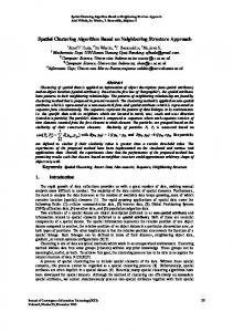
attributes and some are applicable on certain types of data sets, that is, not applicable on arbitrary shape of data [2]. Other methods are based on static nature that is incapable of handling change of dynamic databases and some are not applicable on dense region and presence of physical obstacles. We have studied all possible methods of clustering and their advantages and limitations against the applicability. Our data sources may be tabular file, shape file, comma separated variable (csv) file, rgs file, dbf file, xls file, png file, image file, and so forth. Selection of attributes produces more refined clusters and formation of clusters gives desired results in terms of better efficiency with improved space and time complexity. In Figure 1, we are showing different databases and clusters with application of different methods. These are taken from SEQUOIA 2000 benchmark databases.
2
Mathematical Problems in Engineering 1
0.9
0.9
0.8
0.8
0.7
0.7
0.6
0.6
0.5
0.5 0.4
0.4
0.3
0.3 0.2
0.2
0.1
0.1
0
0
0.1 0.2 0.3 0.4 0.5 0.6 0.7 0.8 0.9
0
1
0
0.1 0.2 0.3 0.4 0.5 0.6 0.7 0.8 0.9
(b)
(a)
(c)
1
0.9
1
0.9
0.8
0.9
0.8
0.7
0.8
0.7
0.7
0.6
0.6
0.6
0.5
0.5
0.5
0.4
0.4
0.4
0.3
0.3
0.3
0.2
0.2
0.2
0.1
0.1
0.1
0
0 0.1 0.2 0.3 0.4 0.5 0.6 0.7 0.8 0.9 1
0
1
0 0.1 0.2 0.3 0.4 0.5 0.6 0.7 0.8 0.9 1
(d)
(e)
0
0 0.1 0.2 0.3 0.4 0.5 0.6 0.7 0.8 0.9 1 (f)
Figure 1: Different shades of spatial data sets from different data collection methods of SPDM.
After detailed study we came to know that still none other than DBSCAN algorithm is yet available for giving better results in the field of clustering. So our area of interest is to design and develop new density based algorithm with better performance. Our improved algorithm will work better in adverse conditions and arbitrary selection of databases. The size and shape and also amount of database will not change the accuracy of creation of clusters. The process of clustering is used for various scientific and social areas [2] like association of business rules, health data, medical imaging, seismology, land treatment, water treatment, cost analysis, and many more. Spatial data mining works on spatial data. Spatial data mining is the discovery of interesting similarities of characteristics and patterns which may exist in large spatial data sets. Spatial clustering is the key concept to get all possible trends and clusters according to given nature of data sets. As discussed above our main objective is to design improved DBSCAN algorithm [3] for spatial data sets. In DBSCAN, the density is measured in the form of point which is obtained by counting the number of points in a region of specified radius around the point. Points with a certain threshold value and densities form the clusters. Major issue in DBSCAN is
the selection of clustering attributes, detection of noise with different densities, and large difference of values of border objects in opposite directions of the same clusters. A point of any object is visited at least once and it may be visited multiple times if it is a candidate of different clusters. This paper is basically designed to give a complete working process of spatial data mining with new ideas of improvement in respect of drawbacks of previous work, that is, DBSCAN. Data collection [4] is a very important and typical process in spatial data mining and knowledge discovery but with the help of efforts of government agencies, scientific needs, and other private sectors it is possible to collect huge data sets of spatial features. For multidimensional data [5], moving objects and dynamic data selection needs new and advance methods of mining and knowledge discovery. To handle such kind of challenges and research activities, spatial data mining has developed as strong tool with geovisualization concept. Significance of Work. Algorithm DBSCAN is improved as IDBSCAN with capacity of recognizing irregular shapes, including concave and nested shapes or satellite images. The IDBSCAN algorithm reduces time of computation as shown in Figure 9 and it is insensitive to bulky amounts of noise.
Mathematical Problems in Engineering A very significant point is that here user does not require domain knowledge of input, that is, amount of clusters to be generated. Primary motive of this paper is to design new and efficient system and algorithms for spatial data mining research, geocomputation, and map analysis. Spatial analysis and mining include various steps of knowledge discovery as data selection, data collection, data cleaning, preprocessing, clustering, classification, and transformation with the help of known and unknown results of knowledge discovery. Various simulative software programs [5, 6] such as GRASS, ERDAS, WEKA, ArcGIS, DIVA-GIS, and MapCalc are available for better experiments. The rest of this paper is organized in the following manner. First we summarize almost all possible and available clustering methods and algorithms with their positive and limited aspects. Point 3 explains the process and meaning of BDSCAN algorithm. Point 4 shows limitations of existing DBSCAN algorithm. Point 5 shows our proposed and improved algorithm (IDBSCAN) which is the novelty of this research article. Point 6 shows analysis of algorithm (IDBSCAN). Point 7 gives idea of results. Finally in point 8 conclusion and future scope is discussed.
2. Related Work and Its Overview In this section we will study the current and previous research work in spatial data mining and knowledge discovery [4]. As we have discussed clustering plays a key role in understanding and application of spatial data in real applications. So we will focus on meaning and methods of clustering in spatial data sets. Recent work in the database community includes density based methods, hierarchical methods, partition based methods, grid based methods, and constraint based methods [3, 7]. A brief idea of each and every method is given here with their positive and limited aspects. 2.1. Density Based Methods. This kind of methods considers clusters as dense region of objects that are different from lower dense regions in the data space. Density based regions are more appropriate and applicable in arbitrary shaped clusters but selection of attributes and selection of clusters with algorithms are more complex. It has the feature to merge two clusters that are sufficiently close to each other. Density biased sampling, DBSCAN (Density Based Spatial Clustering of Applications with Noise), OPTICS (Ordering Points to Identify Clustering Structure), DENCLUE (DENsity CLUstEring), and so forth are example of this method. This method is our major discussion of this research paper so it will be discussed later in detail in the following sections. 2.2. Hierarchical Based Methods. Hierarchical based methods put the data in a tree-like structure. These clusters are classified into agglomerative and divisive hierarchical clustering, depending on whether the decomposition is formed in a bottom-up or top-down manner.
3
8
4
3
8
4
5
5
9
2 1
8
3
3 3
2
4
6
3 1
2
2
7
2 6
3
4
2 2
3
3
9 2
3 5
5
4
6
Clusters = 37
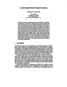
Figure 2: A sample of figure with data points for grid based clustering method.
BIRCH (Balanced Iterative Reducing Clustering and using Hierarchies), CURE (Clustering Using REpresentatives), CHAMELEON, and ORCLUS (arbitrary ORiented projected CLUSter generation) are the basic methods of this category. This (hierarchical methods) can also recognize arbitrary shaped clusters and handles outliers or noise excluding to some special conditions but this method does not work well for special characteristics of individual clusters and it is also time consuming for high dimensional data. 2.3. Partitioning Methods. This method divides 𝑛 objects, which we want to cluster, into 𝑘-partitions, where each partition represents a cluster and 𝑘 is a given parameter. Such algorithms form the clusters to optimize an objective criterion similarity function such as distance as a major parameter [1]. Partitioning methods cover the following five common algorithms: 𝑘-means, 𝑘-medoids, and CLARANS (Clustering Large Applications based upon RANdomized Search). Although partitioning methods are better in generation of clustering results by using 𝑘-mean, 𝑘-medoids are easier to implement but selection of 𝑛 is random so no guarantee of quality of clustering and desired clusters is required in advance which is not more realistic. To handle outliers is also a big problem for such kind of methods. A major drawback of this method is that it is not applicable for large databases. 2.4. Grid Based Methods. Grid based methods summarize the data space into a finite number of cells that form a grid structure on which all of the operations for clustering are performed. These methods are fast in nature and independent of the number of the data objects but dependent on the number of the cells in each dimension in related space of generated results. This method contains the following wellknown algorithms STING (STatistical INformation Grid), wavecluster, CLIQUE (CLustering In QUEst), and STING+. An experimental result is shown in Figure 2.
4 These methods automatically find subspaces of the highest dimensionality and they are insensitive to the order of records but the accuracy of the clustering result may be degraded at certain points. Major applications of such kind of methods are military deployment, situation awareness, and so forth. Most probable results of grid based methods are shown in Figure 2. 2.5. Constrained Based Methods. In our previous paragraphs, we studied that there are so many algorithms and methods to implement and apply clustering in real life and various social purposes. Unfortunately, most of the algorithms are not able to understand or specify real life constraints such as physical obstacles. So it was realized that there should be a method that can handle the concept of clustering in presence of physical obstacles. These are application specific and used as special cases. Constraint based clustering in large databases method gives a novel concept called microclustering and sharing to scale up the algorithm or its working procedure. Other constraints are also discussed in this category as universal, and existential as averaging and summation. COD-CLARANS (Clustering with Obstructed Distance based on CLARANS) is the first clustering algorithm that solves a problem which is known as the problem of clustering with obstacles entities (COE). This method, that is, constraint based clustering, is not well suitable due to NP hard nature of the problems and the fact that there is no guarantee of accuracy of results when number of points is very large, that is, 𝑁. To handle outliers is also a big problem with such kind of methods. 2.6. Spectral Clustering. Spectral clustering is a modern type of clustering method and is being used as a new approach of clustering. For graph and Laplacians based application it is mainly used with standard concept of mathematics and algebra. When constructing similarity graphs the goal is to model the local neighborhood relationships between the data points which is entirely different from 𝑘-means and other methods. The main tool to understand spectral clustering is Laplacians graph matrices. First compute the unnormalized Laplacian 𝐿 from given graph and then determine the eigenvectors of the computed 𝐿 as 𝑢1 , 𝑢2 , . . . , 𝑢𝑛 . Same procedure is used for normalized Laplace 𝐿 and eigenvectors. This property is useful due to nature of change of Laplacian graph method. Output comes in the form of clusters. Consistency of normalized Laplacian data objects is much better than unnormalized ones so we should prefer normalized method of computing of Laplacian 𝐿 and then apply 𝑘-neighborhood method rather than Sigma neighborhood method to select clusters and distance between data points. A very important and popular reason of being successful with spectral clustering is the fact that there is no consideration or assumption on the basis of clusters forms and their numbers in advance. Spectral clustering can solve very simple problems like intertwined spirals and it is used for large data sets, if points are given in the form of sparse. Spectral clustering is used as black box testing method which is the key concept of various clustering and scientific methods.
Mathematical Problems in Engineering
3. Basics of Density Based Clustering (DBSCAN) Clustering and cluster analysis [3, 6, 8] is a widely used method of data analysis, and its function is to organize similar types of set of data items or objects into groups (cluster) so that items in a cluster are similar and different from other clusters. There are many different methods as discussed in our previous paragraphs of this paper about clustering. Density based methods are more effective and efficient for handling large spatial data. We can say that there is no other algorithm that can do what DBSCAN can do in the field of spatial clustering. DBSCAN has altered time to time by various researchers and project agencies in terms of various parameters. Smart definition of parameters gives better results. Selection and application of parameters is a great job in DBSCAN and a situation is shown here. After study of many clustering algorithms [3, 9] we have decided to select and improve DBSCAN algorithm. Some of the reasons why we have selected DBSCAN are its positive points as discussed in the following: (i) It is capable of discovering clusters with arbitrary shapes. (ii) There is no need to predict the number of clusters in advance and hence it is more realistic. (iii) There are greedy methods to replace R∗ -tree data type greedy queries. (iv) Selection and application of attributes is always open to improve time and space complexity. (v) It is robust to outliers and merging is possible with other clusters if they are similar. We have tried to improve DBSCAN in the following directions. The first one is to make DBSCAN handle spatial, nonspatial, and temporal data at a time and distinguish them clearly. The second is to provide a certain density to each cluster so that we can make dense or nondense region accordingly. The third is selection of threshold value 𝜖 which is more realistic and understandable. Some concepts and definitions of DBSCAN which are directly and indirectly related to DBSCAN are explained here: (1) Cluster: in a database with given 𝑁 data objects as 𝐷 = {𝑂1 , 𝑂2 , . . . , 𝑂𝑛 } the procedure of partitioning database 𝐷 into smaller parts which are similar in certain standards as 𝐶 = {𝐶1 , 𝐶2 , . . . , 𝐶𝑖 } is called clustering; 𝐶𝑗 ’s are clusters, where 𝐶𝑗 ≤ 𝐷 (𝑗 = 1, 2, 3, . . . , 𝑖). (2) Neighborhood: a distance function (e.g., Manhattan distance and Euclidean distance) for any two points 𝑝 and 𝑞 denotes dist(𝑝, 𝑞). (3) Eps-neighborhood: the Eps-neighborhood (threshold distance) of a point 𝑝 is defined by {𝑞 ∈ 𝐷 | dist(𝑝, 𝑞) ≤ Eps}. (4) Core object: a point 𝑝 is a core point if at least Minpts points are within distance ∈ of it, and those points are said to be directly reachable from 𝑝. In other words,
Mathematical Problems in Engineering a core object is a point that its neighborhood of a given radius (Eps) has to contain at least a minimum number (Minpts) of other points as shown in Figure 4. (5) Directly density reachable: an object 𝑝 is directly density reachable from the object 𝑞 if 𝑝 is within Epsneighborhood of 𝑞 and 𝑞 is a core object. (6) Density reachable: a point 𝑞 is reachable from 𝑞 if there is a chain 𝑝1 ⋅ ⋅ ⋅ 𝑝𝑛 with 𝑝1 = 𝑝 and 𝑝𝑛 = 𝑞, where each 𝑝𝑖+1 is directly reachable from 𝑝𝑖 with respect to Eps and Minpts, for 1 ≤ 𝑖 ≤ 𝑛, 𝑝𝑖 ∈ 𝐷. (7) Density connected: an object 𝑝 is density connected to object 𝑞 with respect to Eps and Minpts if there is an object 𝑂 ∈ 𝐷 such that both 𝑝 and 𝑞 are density reachable from 𝑜 with respect to Eps and Minpts. (8) Density based clusters: a cluster 𝑐 is nonempty subset of 𝐷 satisfying the following “maximality” and “connectivity” requirements: (i) ∀𝑝, 𝑞: if 𝑞 ∈ 𝐶 and 𝑝 is directly reachable from 𝑞 with respect to Eps and Minpts, then 𝑝 ∈ 𝐶. (ii) ∀𝑝, 𝑞 ∈ 𝐶: 𝑝 is density connected to 𝑞 with respect to Eps and Minpts. (9) Border objects: an object 𝑝 is a border object if it is not a core object but density reachable from another core object. (10) Noise: all points are not reachable from any other point, that is, neither a core point nor density reachable, as shown in Figure 4 as point 𝑁 in blue color. Noise = {𝑝 ∈ 𝐷 | ∀𝑖 : 𝑝 ∉ 𝐶𝑖 }.
4. Problems of Existing Approaches In a nutshell those problems can be summarized as follows [8, 10]: (i) Identification of proper clusters for different types of spatial data sets. (ii) Deficiency of methods in predicting the similarity and number of clusters in advance when the variations of data sets are used. (iii) Difficulty in increasing and decreasing of the interdistance between clusters. (iv) Problem of identification of actual noise points and border objects. (v) Results being not consistent when clusters of different densities are present. (vi) The problem that if the measurements of the neighbor objects have minor differences, then problem of identification of adjacent clusters arises as a major problem; the values of border objects may differ largely from opposite side of same cluster. Situations go uncontrollable if we get data sets with arbitrary shapes like active and inactive volcanoes, polluted areas of Delhi city, and other GIS patterns and outputs of these data
5 sets produce very adjacent and close clusters with overlapping boundaries [6, 7]. A result of DBSCAN is shown in Figure 4. Different results are also shown in Figure 1.
5. Proposed Solution with Development of New Algorithm (IDBSCAN) Our research object is to get solutions of given problem in Section 4. Here we have decided to design and develop new methods, techniques, and algorithms to find efficient, effective robustness to noise and outliers, tuning of proper parameters, and so forth. This can be achieved by considering only important components of existing algorithm and selection of data sets. However DBSCAN requires two important parameters as follows [2, 10, 11]: (i) Eps is the radius that represents spatial attribute (latitude and longitude) that delimitates the neighborhood area of a point. (ii) Minpts is the minimum number of points that must exist in the Eps-neighborhood. This method is highly dependent on parameters provided by the users and expensive in computation when size of input data is unlimited. Our proposed algorithm I-DBSCAN requires 5 parameters as follows: 𝑘 is the neighbor list size. Eps1 is distance for spatial data objects. Eps2 is distance measure for nonspatial data objects. Minpts is minimum number of points within a cluster and Eps1 and Eps2. 𝜖 is a threshold value. IDBSCAN works as follows. The algorithm begins with any arbitrary point, 𝑝, from database 𝐷 and retrieves all points density reachable from 𝑝 wrt to Eps and Minpts. The retrieval of density reachable objects is performed by iteratively collecting directly density reachable objects. If 𝑝 is a core point (i.e., |𝑁Eps (𝑝)| ≥ Minpts), then 𝑝 and all points that are density reachable are collected in one cluster. If 𝑝 is a border point and no points are density reachable as per definition from 𝑝 then algorithm explores next point of the database. If 𝑝 is not a core point, then 𝑝 is considered as outlier and discarded later as noise if it does not belong to any cluster. The algorithm terminates when no new points can be assigned to any cluster. These attributes are described in Figure 3 and definitions from 1 to 10. Flowchart of IDBSCAN algorithm is depicted in Figure 5 for better understanding of IDBSCAN and in Algorithm 1. Use of stack is necessary to get density reachable objects from directly density reachable objects. If two clusters 𝐶1 and 𝐶2 have very less distance between them, a point 𝑝 may belong to both clusters 𝐶1 and 𝐶2 . Here this point will be considered as border point for both clusters and finally algorithm assigns this point 𝑝 to the first discovered clusters. So in this way we can overcome the problem of outliers and border object.
6
Mathematical Problems in Engineering
N A
C
B
Figure 3: Points with red color are core points; points B and C with yellow color are density reachable and the point with blue color N is a form of noise.
Input: (1) A set of 𝑁 objects in a spatial area as 𝐷 = {𝑂1 , 𝑂2 , . . . , 𝑂𝑛 ) (2) 𝐾, The neighbor list size (3) Eps points –radius for spatial and non-spatial data objects (4) Minpts- The minimum number of points that must exist in the Eps neighborhood (5) 𝜖- Threshold value to be included in a cluster. Output: Clusters with their core objects and noise points as 𝐶 = {𝑐1 , 𝑐2 , . . . , 𝑐𝑛 }. Method: (1) Set cluster layer = 0; (2) Initialize a loop for selecting objects from the given data base 𝐷 For 𝑖 = 1 to 𝑛 do //select an arbitrary object 𝑂𝑖 and check if it is visited or not If 𝑜𝑖 does not belong to any cluster, then Move forward to process next point 𝑃 = process neghbors as region query(𝑂𝑖 , Eps); If sizeof(𝑝) < Minpts then Mark next point(𝑜𝑖 ) as noise Else Cluster layer = Cluster layer + 1; //Increase the cluster number For 𝑗 = 1 to sizeof(𝑝) // set cluster number to all points in 𝐷 End (of marking) Expand cluster by pushing all points to 𝑝 Expand cluster(push() all objects to 𝑃) While (𝐷! = empty()) //Repeat the process while database is not empty Object = pop(); //Apply pop operation on current object 𝑄 = process neighbors(current point, Eps1, Eps2) //spatial and non spatial objects distance If 𝑄 ≥ Minpts then For 𝑘 = 1 to 𝑂𝑛 in 𝑄 If (𝑜 is not visited and not identified as a noise and sizeofneghborpts ≥ 𝜖) then Add 𝑂 with current cluster End if End if Push(𝑜) End for End for Region Query(𝑝, Eps) End while End of algorithm Return all points with cluster number and Eps-neighborhood. Algorithm 1: Algorithm IDBSCAN.
Mathematical Problems in Engineering
7
35
Start
30
Y coordinates
25
Set D = Data set
20 Loop
15 10
Select an arbitrary point P from D
5 0
0
5
10
15 20 X coordinates
25
30
Cluster 0 Cluster 1 Cluster 2
Figure 4: Result of DBSCAN algorithm for different data sets with different clusters.
Is P a core point?
This session analyzes the working performance and its complexities for the new designed algorithm. Major notation used in this algorithm is number of objects 𝑁 in the database 𝐷 and 𝑘 is the size of list. A well-structured and stored database gives better results. So performing query operation and accessing data from database is a major role playing function to optimize overall performance. Indexing of data and selection of data are also a matter of consideration. It has been proved that sequence of selection of data points does not affect the time complexity [10]. Step by step analysis is given here: (1) Initialization of cluster will execute only once, that is, +1. (2) Counting of loop will take 𝑁 + 1 times. (3) Comparison step < 𝑁 + 1 and hence total time 𝑁 + 1. (4) Discarded or noise points decrease the number of visits in logarithmic form so size of list decreased by log 𝑁 time. (5) Again increment step is executed 𝑛 times. (6) Finally the total time is calculated as 1 + (𝑁 + 1) + 𝑁 ⋅ log 𝑁 = 𝑂(𝑁 log 𝑁).
No
Is P a border point?
No Yes
6. Analysis of Performance of Algorithm
No
Identify all density reachable points with respect to EPS1 and EPS2 with Minpts
35
Cluster formed with ID
Yes Detect as noise and discard
Have all points visited, for example, D = 𝜙?
Yes End
Figure 5: Flowchart of given pseudocode of IDBSCAN algorithm.
Well-known indexing technique R-Tree and order of query is also helpful in reduction of time unit.
7. Results and Discussion Sources of data collection are satellite images, medical images, geographic images, and various research and project agencies [5, 12]. The data is collected in the form of .png, .shp, .tab, .dbf, .txt, .csv, .rgs, .tif, .xls, and so forth. Results and performance are shown in Figures 6, 7, 8, and 9.
Figure 6: Satellite image of Mumbai city.
With application of density based clustering (IDBSCAN) on image of Figure 6, we get the result shown in Figure 7. For Figure 7 we have used a different color for identification of noise as blue point and black point as input data and
8
Mathematical Problems in Engineering 25
Run time (sec)
20
15
10
5
Figure 7: Output of Figure 6 in clustered form with the application of IDBSCAN.
0
0
500
1000
1500 2000 2500 Number of data sets
3000
3500
4000
IDBSCAN DBSCAN
Figure 9: Working performance of DBSCAN and IDBSCAN.
Figure 8: This form of screenshot for given data in Table 1 is generated from SPDM Software DIVA-GIS in the form of .shp file format.
red point is used to represent core point. Other details are as follows. The results with Eps set to 0.0045 and MinPts = 7 give 3700 clusters, and 488,763 out of the total of 710,148 points end up in a cluster. Data collected from different research agencies are available but an example is shown here [12–14] in table form with spatial attributes. The algorithm was implemented as per sequence of pseudocode in c language and then from the program [15], input and output forms are given as follows: (0,100)(0,200)(0,275)(100,150)(200,100)(250,200)(0, 300)(100,200)(600,700)(650,700)(675,710)(675,720) (50,400). Eps = 100.0 Minpts = 3 Output of this input may be as Cluster 1- (0,100)(0,200)(0,275)(100,150)(0,300)(100, 200). Cluster 2- (600,700)(650,700)(675,700)(675,710) (675,720) Noise points will be identified as – (200,100)(250,200) (50,100). From the above discussion, pictorial data and textual data output may be different but anyhow results are based on working of algorithm of density based concept. IDBSCAN is
applicable for both and above described formats of data or file types. It has been noticed that, for large data size, generation of results degraded in the form logarithmic nature. Another screenshot is given here for estimation of performance. It is shown in Figure 9. As shown in Figure 9 the performance of IDBSCAN is better in terms of data units and run time. IDBSCAN creates a linear increase in computing time related to the number of points in database. Figure 9 is generated on various size of data units and results are computed at general computer machine. Limitation and future aspects are mentioned in the next phase. A logical comparison between DBSCAN and IDBSCAN may be summarized as follows [16]: (1) DBSCAN is density based approach but it is weak in density reachability of a point to others, whereas IDBSCAN is more accurate in density reachability approach. (2) DBSCAN can find arbitrary shaped clusters but it is weak to separate those clusters who are very close (but not overlapped) where our IDBSCAN gives better performance for close points having dissimilar properties and very close clusters at boundary, that is, border points. (3) Both do not require number of clusters (𝑘) in advance but DBSCAN cannot cluster data sets well with large differences in densities, whereas IDBSCAN can do it properly. (4) DBSCAN requires 2 parameters while IDBSCAN requires 5 parameters. (5) Outlier detection is much better in IDBSCAN. (6) Computational difference is given in Figure 9.
Mathematical Problems in Engineering
9
Table 1: Data collected from government agencies for traffic controller and land use. Category Loading zone Loading zone Loading zone Loading zone Loading zone Loading zone Loading zone Loading zone Loading zone Loading zone Loading zone Loading zone Loading zone Loading zone
Type Commercial and passenger Commercial and passenger Commercial and passenger Commercial and passenger Commercial Commercial and passenger Commercial and passenger Commercial and passenger Commercial and passenger Commercial and passenger Commercial and passenger Commercial and passenger Commercial and passenger Commercial
SHAPE AREA 114.3193935 36.30879624 15.1329729 46.3432375 22.23059338 33.66437817 79.2862063 28.21015191 15.94021067 58.98030586 74.1102419 30.57185763 34.18517554 22.73934692
SHAPE LEN 102.6164835 35.57997895 19.40907856 46.33549105 21.35827733 34.46180399 80.89769525 26.75254133 18.61440417 67.1753521 58.92336639 33.71165202 35.05289705 30.41373818
POINT 𝑋 153.0301 153.028 153.0273 153.0299 153.025 153.0269 153.0303 153.0298 153.0295 153.0239 153.0204 153.0286 153.0259 153.0289
POINT 𝑌 −27.4672 −27.4716 −27.4721 −27.4687 −27.4685 −27.4714 −27.4691 −27.4695 −27.471 −27.4726 −27.4768 −27.4723 −27.4735 −27.4675
8. Conclusion and Future Work
References
In this research paper, we introduced a new density based clustering algorithm IDBSCAN that is designed by modification of DBSCAN clustering algorithm. A detailed study may be summarized as follows:
[1] M. Ester, A. Frommelt, H.-P. Kriegel, and J. Sander, “Spatial data mining: database primitives, algorithms and efficient DBMS support,” Data Mining and Knowledge Discovery, vol. 4, no. 2, pp. 193–216, 2000. [2] O. R. Za¨ıane and C.-H. Lee, “Clustering spatial data in the presence of obstacles: a density-based approach,” in Proceedings of the International Database Engineering and Applications Symposium (IDEAS ’02), pp. 214–223, July 2002. [3] M. Hemalatha, M. Naga, and N. Saranya, “A recent survey of knowledge discovery in spatial data mining,” International Journal of Computer Science, vol. 8, no. 3, article 2, 2011. [4] J. K. Berry, Map Analysis: Procedures and Applications in GIS Modeling, 2004. [5] http://www.esri.com/. [6] R. H. G¨uting, “An introduction to spatial database systems,” The VLDB Journal, vol. 3, no. 4, pp. 357–399, 1994. [7] D. Birant and A. Kut, “ST-DBSCAN: an algorithm for clustering spatial-temporal data,” Data & Knowledge Engineering, vol. 60, no. 1, pp. 208–221, 2007. [8] Z. Aoying and Z. Shuigeng, “Approaches for scaling DBSCAN algorithm to large spatial databases,” Journal of Computer Science and Technology, vol. 15, no. 6, pp. 509–526, 2000. [9] R. Ng and J. Han, “Effective and efficient clustering methods for spatial data mining,” Tech. Rep. 94-13, University of British Columbia, Vancouver, Canada, 2001. [10] R. Muetzelfeldt and M. Duckham, Dynamic Spatial Modeling in the Similie Visual Modeling Environment, chapter 17, John Wiley & Sons, New York, NY, USA, 2005. [11] A. Galton, Qualitative Spatial Change, Oxford University Press, Oxford, UK, 2000. [12] http://www.kdnuggets.com/. [13] http://ftp2.cits.rncan.gc.ca/. [14] http://www.geodata.gov.gr/. [15] B. Kazar, S. Shekhar, D. Lilja, and D. Boley, “A parallel formulation of the spatial autoregression model for mining large geo-spatial datasets,” in Proceedings of the SIAM International Conference on Data Mining Workshop on High Performance and Distributed Mining (HPDM ’04), April 2004. [16] C. Fraley and A. E. Raftery, “Model-based clustering, discriminant analysis, and density estimation,” Journal of the American Statistical Association, vol. 97, no. 458, pp. 611–631, 2002.
(i) The first reason is to modify DBSCAN to cluster spatial data of any kind such as .png, .dbf, .csv, .rgs, .xls, .scr, and .txt. (ii) This algorithm can find a cluster completely surrounded by different and very close clusters of different densities. (iii) The second modification is about using five parameters instead of two as in DBSCAN. (iv) The effectiveness of proposed algorithm was demonstrated by using a real and synthetic database. (v) This paper gives an opportunity to apply clustering algorithm over new types of data and new application areas such as moving objects and trajectories, spatially embedded social networks, and geocoded multimedia and web based data. From experimental results it has been found that very large and dense data needs higher computational power. So, for further extension it may be designed for parallel and multithreading concept. Experimental results are very relevant according to our objective and improved algorithm. Selection of Eps and Minpts with threshold Δ𝜖 may be more intelligent and heuristically efficient. Scope of designing of new spatial data mining algorithm is still considerable for neighborhood objects and graphs.
Competing Interests The authors declare that there are no competing interests regarding the publication of this manuscript.
Advances in
Operations Research Hindawi Publishing Corporation http://www.hindawi.com
Volume 2014
Advances in
Decision Sciences Hindawi Publishing Corporation http://www.hindawi.com
Volume 2014
Journal of
Applied Mathematics
Algebra
Hindawi Publishing Corporation http://www.hindawi.com
Hindawi Publishing Corporation http://www.hindawi.com
Volume 2014
Journal of
Probability and Statistics Volume 2014
The Scientific World Journal Hindawi Publishing Corporation http://www.hindawi.com
Hindawi Publishing Corporation http://www.hindawi.com
Volume 2014
International Journal of
Differential Equations Hindawi Publishing Corporation http://www.hindawi.com
Volume 2014
Volume 2014
Submit your manuscripts at http://www.hindawi.com International Journal of
Advances in
Combinatorics Hindawi Publishing Corporation http://www.hindawi.com
Mathematical Physics Hindawi Publishing Corporation http://www.hindawi.com
Volume 2014
Journal of
Complex Analysis Hindawi Publishing Corporation http://www.hindawi.com
Volume 2014
International Journal of Mathematics and Mathematical Sciences
Mathematical Problems in Engineering
Journal of
Mathematics Hindawi Publishing Corporation http://www.hindawi.com
Volume 2014
Hindawi Publishing Corporation http://www.hindawi.com
Volume 2014
Volume 2014
Hindawi Publishing Corporation http://www.hindawi.com
Volume 2014
Discrete Mathematics
Journal of
Volume 2014
Hindawi Publishing Corporation http://www.hindawi.com
Discrete Dynamics in Nature and Society
Journal of
Function Spaces Hindawi Publishing Corporation http://www.hindawi.com
Abstract and Applied Analysis
Volume 2014
Hindawi Publishing Corporation http://www.hindawi.com
Volume 2014
Hindawi Publishing Corporation http://www.hindawi.com
Volume 2014
International Journal of
Journal of
Stochastic Analysis
Optimization
Hindawi Publishing Corporation http://www.hindawi.com
Hindawi Publishing Corporation http://www.hindawi.com
Volume 2014
Volume 2014