Improved HAR Inference. Using Power Kernels without Truncation". Peter C. B. Phillips. Cowles Foundation, Yale University,. University of Auckland & University ...
IMPROVED HAR INFERENCE USING POWER KERNELS WITHOUT TRUNCATION
By Peter C.B. Phillips, Yixiao Sun and Sainan Jin
June 2005
COWLES FOUNDATION DISCUSSION PAPER NO. 1513
COWLES FOUNDATION FOR RESEARCH IN ECONOMICS YALE UNIVERSITY Box 208281 New Haven, Connecticut 06520-8281 http://cowles.econ.yale.edu/
Improved HAR Inference Using Power Kernels without Truncation
Peter C. B. Phillips Cowles Foundation, Yale University, University of Auckland & University of York Yixiao Sun Department of Economics University of California, San Diego and Sainan Jin Guanghua School of Management Peking University
November 29, 2004
Phillips thanks the NSF for partial research support under Grant No. SES 04-142254.
ABSTRACT Employing power kernels suggested in earlier work by the authors (2003), this paper shows how to re…ne methods of robust inference on the mean in a time series that rely on families of untruncated kernel estimates of the long-run parameters. The new methods improve the size properties of heteroskedastic and autocorrelation robust (HAR) tests in comparison with conventional methods that employ consistent HAC estimates, and they raise test power in comparison with other tests that are based on untruncated kernel estimates. Large power parameter ( ) asymptotic expansions of the nonstandard limit theory are developed in terms of the usual limiting chi-squared distribution, and corresponding large sample size and large
asymptotic expansions of the …nite sample distribution of
Wald tests are developed to justify the new approach. Exact …nite sample distributions are given using operational techniques. The paper further shows that the optimal
that
minimizes a weighted sum of type I and II errors has an expansion rate of at most O T 1=2 and can even be O (1) for certain loss functions, and is therefore slower than the O T 2=3 rate which minimizes the asymptotic mean squared error of the corresponding long run variance estimator. A new plug-in procedure for implementing the optimal
is suggested.
Simulations show that the new plug-in procedure works well in …nite samples.
JEL Classi…cation: C13; C14; C22; C51 Keywords: Asymptotic expansion, consistent HAC estimation, data-determined kernel estimation, exact distribution, HAR inference, large loss function, power parameter, sharp origin kernel.
asymptotics, long run variance,
1
Introduction
Seeking to robustify inference, many practical methods in econometrics now make use of heteroskedasticity and autocorrelation consistent (HAC) covariance matrix estimates. Most commonly used HAC estimates are formulated using conventional kernel smoothing techniques (for an overview, see den Haan and Levin (1997)), although quite di¤erent approaches like wavelets (Hong and Lee (2001)) and direct regression methods (Phillips (2004)) have recently been explored. While appealing in terms of their asymptotic properties, consistent HAC estimates provide only asymptotic robustness in econometric testing and …nite sample performance is known to be unsatisfactory in many cases, but especially when there is strong autocorrelation in the data. HAC estimates are then biased downwards and the associated tests are liberal-biased. These size distortions in testing are often substantial and have been discussed extensively in recent work (e.g., Kiefer and Vogelsang (2003) and Sul, Phillips and Choi (2003)). Robusti…cation in regression testing is achieved by the use of a test statistic that is asymptotically pivotal under a general maintained hypothesis for the regression components. Consistent HAC estimation is not necessary for this purpose and, indeed, any procedure that scales out the e¤ects of the nuisance parameters in the test statistics will work. Kiefer, Vogelsang and Bunzel (2000, hereafter KVB) suggested the use of untruncated, inconsistent kernel estimates in the construction of test statistics and showed that the limit theory is nuisance parameter free but no longer standard normal or chi-squared. Work on related procedures has been done by Vogelsang (2003), Kiefer and Vogelsang (2002a, 2002b, 2003; hereafter KV) and by the present authors (2003a & 2003b; hereafter PSJa & PSJb ). These techniques may be grouped with conventional HAC procedures as having the same goals of robust inference and the term heteroskedastic and autocorrelation robust (HAR) methods has been used to collectively describe them (Phillips, 2004). Inconsistent covariance matrix estimates play an interesting role in improving the size properties of tests, essentially because they preserve in the limit theory the …nite sample randomness of the denominator in the conventional t-ratio. In this respect, these tests behave in large samples more like their …nite sample analogues than the conventional asymptotic normal and chi-squared tests, for which the denominator is non-random. In
1
the case of the Gaussian location model, Jansson (2004) showed that the KVB test statistic is closer to its limit distribution in the precise sense that the error in the rejection probability (ERP) is of order O T
1 log T
for sample size T under the null, whereas
the corresponding ERP for a test based on a conventional consistent HAC estimate is at most of order O(T
1=2 );
as shown in Velasco and Robinson (2001). While tests such
as KVB typically have better size than those that use HAC estimators, there is also a clear and compensating reduction in power. The challenge is to develop test procedures with size improvements like those of KVB, while retaining the good power properties of conventional tests based on HAC estimators. The present paper confronts this challenge by developing a procedure that combines the use of untruncated kernels, as in KVB, with a re…nement that enables the use of critical values that appropriately correct those of the limit theory for conventional tests based on consistent HAC estimators, while at the same time enhancing the test power of the KVB test. The class of HAR tests considered here involve the use of a power kernel suggested by the authors in other work (2003a) and this class includes both consistent and inconsistent HAC estimates, depending on whether the power parameter, ; is …xed or passes to in…nity as T ! 1: When
! 1; the …rst order limit theory corresponds
to that of a test based on conventional consistent HAC estimation, whereas for
…xed,
the limit theory is nonstandard, as in the case of the KVB test. The mechanism for making improvements in both size (compared with asymptotic normal tests) and power (compared with the KVB test) is to use a test statistic for a moderate value of
for which
the critical values can be obtained from the appropriate nonstandard limit distribution, which is nuisance parameter free. It is shown here how these critical values may be very well approximated using an asymptotic expansion of the limit distribution about its limiting chi-squared distribution. This version of the procedure has the advantage of being easily implemented and does not require the use of tables of nonstandard distributions. This re…nement improves test size in the same manner as the KVB test, and is justi…ed in the present paper by asymptotic expansions of both the non-standard limit distribution as
! 1 and the …nite sample distribution as T ! 1 and
! 1: The …rst expansion
can be regarded as a high order expansion under the sequential limit in which T ! 1 …rst followed by
! 1: The second expansion is a high order expansion under the joint limit
in which T ! 1 and
! 1 simultaneously. Corresponding asymptotic expansions of 2
the power functions indicate that for typical economic time series test power increases as increases. Finite sample improvements in test power over other tests with untruncated kernels like the KVB test have been noted in simulations reported in other work by the authors (2003a, 2003b) and in independent work by Ravikumar, Ray and Savin (2004) using the methods of PSJb . The asymptotic expansions given in the present paper help to explain these power improvements. A further contribution of the present paper is to use these asymptotic expansions to suggest a practical procedure for test implementation which optimally balances the type I and type II errors. The type I error is measured by using the …rst correction term in the asymptotic expansion of the …nite sample distribution of the test statistic about its nonstandard limit distribution. This term is of order O ( =T ) and it increases in magnitude as
increases for any given T . Similarly, the expansions under the local
alternative reveal that in general the type II error decreases as order in the asymptotic expansion, increasing
increases. Thus, to this
reduces the type II error but also increases
the type I error. Since the desirable e¤ects on the two types of errors generally work in opposing directions, we construct a loss function criterion by taking a weighted sum of the two types of errors and show how
may be selected in such a way as to optimize the
criterion. This approach gives an optimal most
opt
which generally has an expansion rate of at
= O T 1=2 and which can even be O (1) for certain loss functions. This rate is
less than the optimal rate of O T 2=3 that applies when minimizing the asymptotic mean squared error of the corresponding HAC variance estimate (c.f., PSJa ). Thus, optimal values of
for HAC standard error estimation are larger as T ! 1 than those which are
most suited for statistical testing. The …xed
rule is obtained by attaching substantially
higher weight to the type I error in the construction of the loss function. This theory therefore provides some insight into the type of loss function for which there is a decision theoretic justi…cation for the use of …xed
rules in econometric testing. These conclusions
are also relevant to the use of untruncated kernel estimates in econometric testing of the type suggested in KV (2003). The plan of the paper is as follows. Section 2 overviews the class of power kernels that will be used in the present paper’s development and reviews some …rst order limit theory for Wald type tests as T ! 1 with the power parameter
…xed and as
! 1. Section
3 derives an exact distribution theory using operational techniques. Section 4 develops 3
an asymptotic expansion of the non-standard limit distribution under the null hypothesis as the power parameter
! 1 about the usual limiting chi-squared distribution. The
second order term in this asymptotic expansion delivers a correction term that can be used to adjust the critical values in the usual chi-squared test. An asymptotic expansion of the local power function is also given. Section 5 develops comparable expansions of the …nite sample distribution of the statistic as T ! 1 for a …xed and
and as both T ! 1
! 1. This expansion validates the use of the corrected critical values in practical
work. Section 6 proposes a selection rule for
that is suitable for implementation in
semiparametric testing. This criterion optimizes a loss function that is constructed to balance higher order approximations to the type I and type II errors. Section 7 reports some simulation evidence on the performance of the new procedures. Section 8 concludes and discusses the implications of the results for applied work. Proofs and additional technical results are in the Appendix.
2
HAR Inference for the Mean
Throughout the paper, we focus on the inference about yt =
+ ut ;
in the location model:
t = 1; 2; :::; T;
(1)
where ut is zero mean process with a nonparametric autocorrelation structure. The nonstandard limiting distribution in this section and its asymptotic expansion in Section 4 apply to general regression models under certain conditions on the regressors, see PSJa : However, the asymptotic expansion of the …nite sample distribution in Section 5 applies only to the location model. A possible extension is discussed in Section 8. The OLS estimation of
gives T X ^=Y = 1 yt T t=1
and the scaled estimation error is p where St =
Pt
=1 u
: Let u ^ =y
T(^
1 ) = p ST ; T
(2)
^ be the demeaned time series and S^t = Pt u =1 ^ be
the corresponding partial sum process.
4
The following condition is commonly used to facilitate the limit theory (e.g., KVB, PSJa ; and Jansson, 2004). Assumption 1 S[T r] satis…es the functional law T
1=2
S[T r] ) !W (r);
r 2 [0; 1]
where ! 2 is the long run variance of ut and W (r) is the standard Brownian motion. Under Assumption 1, T
1=2 ^ S[T r]
) !V (r);
r 2 [0; 1] ;
(3)
where V is a standard Brownian bridge process, and p
T(^
) ) !W (1) = N (0; ! 2 );
(4)
which provides the usual basis for robust testing about : It is the standard practice to estimate ! 2 using kernel-based nonparametric HAC estimators that involve smoothing and truncation lag covariances. When ut is stationary with spectral density fuu ( ) ; the long run variance (LRV) of ut is !2 =
0+2
1 X
(j) = 2 fuu (0) ;
(5)
j=1
where (j) = E(ut ut ! ^ 2 (M ) =
HAC estimates of ! 2 typically have the following form 8 T < 1 PT j u u X1 for j 0 j t=1 t+j t T k( )^ (j); ^ (j) = P : 1 T M ut+j ut for j < 0 j ):
j= T +1
T
(6)
t= j+1
involving the sample covariances ^ (j): In (6), k( ) is some kernel function, M is a bandwidth parameter, and consistency of ! ^ 2 (M ) requires M ! 1 and M=T ! 0 as T ! 1 (e.g. Andrews (1991), Andrews and Monahan (1992), Hansen (1992), Newey and West (1987,1994), de Jong and Davidson (2000)). Jansson (2002) provides a recent overview and weak conditions for consistency of such estimates. To test the null H0 :
=
0
against H1 :
6=
0;
the standard approach relies on a
t-ratio statistic of the form t!^ (M ) = T 1=2 ( ^ 5
! (M ) 0 )=^
(7)
which is asymptotically N (0; 1). Use of t!^ (M ) is convenient empirically and therefore widespread in practical work, in spite of well-known problems of size distortion in inference. In a series of papers, KVB and KV propose the use of kernel-based estimators of ! 2 in which M is set equal to the sample size T or proportional to T . These estimates are inconsistent and tend to random quantities instead of ! 2 ; so the limit distribution of (7) is no longer standard normal. Nonetheless, use of these estimates results in valid asymptotically similar tests. In related work, PSJa and PSJb propose the use of estimates of ! 2 based on power kernels without truncation, so that M = T again. For instance, in PSJa a class of sharp origin kernels were constructed in this way by taking an arbitrary power
1 of the
usual Bartlett kernel, giving 8 < (1 jxj) ; jxj 1 k (x) = : 0; jxj > 1
2 Z+ :
for
(8)
We will focus on the sharp origin kernels in the rest of the paper. Using k in (6) and letting M = T gives HAC estimates of the form 2
! ^ =
T X1
j T
k
j= T +1
Under Assumption 1, ! ^ 2 ) !2
; where
=
The associated t statistic is given by
R1R1 0
t (^ ! ) = T 1=2 ( ^ When the power parameter
^ (j):
0
(9)
k (r
! 0 )=^
s)dV (r)dV (s).
:
(10)
is …xed as T ! 1; PSJa showed that under Assumption 1
the t -statistic has the nonstandard limit distribution: 1=2
t (^ ! ) ) W (1)
(11)
under the null and t (^ ! ) ) ( + W (1)) under the local alternative H1 : When
=
0
+ cT
1=2 ;
1=2
where
;
(12)
= c=!:
is sample size dependent and satis…es 1= + ( log T ) =T ! 0, PSJa showed
that ! ^ is consistent. In this case, the t -statistic has conventional normal limits: under the null t (^ ! ) ) W (1) =d N (0; 1); and under the local alternative t (^ ! ) ) + W (1): 6
Thus, the t -statistic has nonstandard limit distributions arising from the random limit of the HAC estimate ! ^ when However, as
is …xed as T ! 1; just as the KVB and KV tests do.
increases, the e¤ect of this randomness diminishes, and when
! 1 the
limit distributions approach those of conventional regression tests with consistent HAC estimates. The mechanism we develop for making improvements in size without sacri…cing much power, is to use a test statistic constructed with ! ^ based on a moderate value of : The critical values of this test can be obtained from the …xed
limit theory given above.
Alternatively, they can be based on an accurate but simple asymptotic expansion of that distribution about its limiting chi-squared distribution that applies as
! 1. This
expansion is developed in Section 4.
3
Probability Densities of the Nonstandard Limit Distribution and the Finite Sample Distribution
This section develops some useful formulae for the probability densities of the …xed
limit
theory and the exact distribution of the test statistic. First note that in the limit theory of the t-ratio test, W (1) is independent of 1=2
the conditional distribution of W (1) 1:
We can write
pdf of t = W (1)
= 1=2
given
, so
is normal with zero mean and variance
(V) where the process V has probability measure P (V) : The
can then be written in the mixed normal form as Z pt (z) = N 0; 1 dP (V) :
(13)
(V)>0
For the …nite sample distribution of tT = t (^ ! ), we assume that ut is a Gaussian p process. Since ut is in general autocorrelated, T ( ^ ) and ! ^ are statistically dependent. To …nd the exact …nite sample distribution of the t-statistic, we decompose ^ and ! ^ into statistically independent components. Let u = (
0 1 ; :::uT ) ;
and
is ~ = lT0
T
= var(u): Then the GLS estimator of ^
where u ~ = (I
lT lT0
1 T
lT
= ~ 1 0 lT
1 T
+ lT0 lT
y = (y1 ; :::; yT ); lT = (1; :::; 1)T 1 T
lT
1 0 lT
1 T
y and
1 0 lT u ~
)u; which is statistically independent of ~
7
(14) :
Therefore the t-statistic can be written as p l0 u ~ T(~ ) +p T tT = ! ^ (^ u) T! ^ (~ u) lT (lT0 lT )
It is easy to see that u ^= I
1 l0 T
(15)
lT (lT0 lT )
u= I
1 l0 T
u ~: As consequence,
the conditional distribution of tT given u ~ is 1
T lT0 T 1 lT p ; (^ ! (~ u))2 T! ^ (~ u) ~ lT0 u
N
!
:
(16)
Letting P (~ u) be the probability measure of u ~; we deduce that the probability density of tT is ptT (z) =
Z
=E
p
N (
~ lT0 u T! ^ (~ u)
p
N
;
lT0 u ~ T! ^ (~ u)
T lT0
1 T
lT
(^ ! (~ u))2 ;
T lT0
1 T
lT
1
! 1
(^ ! (~ u))2
dP (~ u)
!)
;
(17)
which is a mean and variance mixture of normal distributions. Using u ~ s N 0;
T
lT lT0
1 T
lT
1 0 lT
and employing operational techniques along
the lines developed in Phillips (1993), we can write expression (17) in the form " !Z # 1 T lT0 T 1 lT lT0 @q z0 u ~ ptT (z) = N p ; e dP (~ u) T! ^ (@q) (^ ! (@q))2 q=0 " ! n o # 1 1 0 0 1 0 1 0 0 T lT T lT lT @q q lT q T lT (lT T lT ) = N p e : ; T! ^ (@q) (^ ! (@q))2 q=0
(18)
This provides a general expression for the …nite sample distribution of the test statistic tT under Gaussianity.
4
Expansion of the Nonstandard Limit Theory
This section develops asymptotic expansions of the limit distributions given in (11) and (12) as the power parameter
! 1: These expansions can be taken about the relevant
central and noncentral chi-squared limit distributions that apply when
! 1; corre-
sponding to the null and alternative hypotheses. The expansions of the nonstandard limit distributions are of some independent interest. For instance, they can be used to deliver correction terms to the limit distributions 8
under the null, thereby providing a mechanism for adjusting the nominal critical values provided by the usual chi-squared distribution. The latter correspond to the critical values that would be used for tests based on conventional consistent HAC estimates. As we shall see, when the O (1= ) correction on the nominal chi-squared asymptotic critical value is implemented using this asymptotic expansion, the resulting expression provides an asymptotic justi…cation for the continued fraction approximation suggested in PSJa for practical testing situations. 2 1
Let D( ) be the cdf of a P
n
Observe that
W (1)
variate, then o z = P W 2 (1)
1=2
= E D(z 2
z2
) :
(19)
is a quadratic functional of a Gaussian process whose moments exist to
all orders. It follows that we may develop an expansion of E D(z 2 moments of
where
=E(
) = =( + 2); and
2
= var (
) in terms of the ) : In particular, we
have ED(z 2 as
) = D(
1 z 2 ) + D00 ( 2
z 2 )z 4 E (
)2 + O E(
)3
! 1; where the O ( ) term holds uniformly for any z 2 [Ml ; Mu ]
(20)
R+ and Ml and
Mu may be chosen arbitrarily small and large, respectively. As shown in Lemma 7 in the )j = O(1=
appendix, E(
j 1)
as
! 1; so that (20) gives an asymptotic series
representation in increasing powers of 1 of the limit distribution (19). R1R1 In fact, as shown in PSJa , = 0 0 k (r; s)dW (r)dW (s); where k (r; s) is de…ned by
k (r; s) = k (r
s)
Z
0
1
k (r
t)dt
Z
0
1
k (
s)d +
Z
0
1Z 1
k (t
)dtd :
0
The function k (z) is continuous, symmetric and positive semi-de…nite, which guarantees the positive semi-de…niteness of kernel HAC estimators de…ned as in (9), c.f. Newey and West (1987), Andrews (1991). The positive semi-de…niteness of k (z) inherits from that of k(z); see Sun (2004) for a proof. The positive semi-de…niteness enables the use of Mercer’s theorem (e.g., see Shorack and Wellner (1986)) so that k (r s) can be represented as P k (r s) = 1 n=1 n fn (r)fn (s); where n > 0 are the eigenvalues of the kernel and fn (x) R1 are the corresponding eigenfunctions, i.e. n fn (s) = 0 k(r s)fn (r)dr: Now with
n
> 0; k (r; s) is also positive semi-de…nite. This is because k (r; s) can
9
be written as k (r; s) =
1 X
n gn (r)gn (s)
for any (r; s) 2 [0; 1]
n=1
R1
where gn (r) = fn (r)
0
fn ( )d ; and
n
[0; 1]:
(21)
and fn ( ) are eigenvalues and eigenfunctions of
s): As a consequence, for any function q(x) 2 L2 [0; 1]; we have
k (r
Z
0
1Z 1
q(r)k (r; s)q(s)drds =
0
1 X
n
n=1
Z
2
1
(22)
0
Thus, by Mercer’s theorem, k (r; s) has the representation k (r; s) = in terms of
0:
gn (r)q(r)dr
P1
n=1
n fn (r)fn (s)
> 0; the eigenvalues of k (r; s); and fn (x); the corresponding eigenP 2 functions. Using this representation, we can easily show that = 1 n=1 n Zn ; where n
Zn s iidN (0; 1) for n
1. Therefore, the characteristic function of
n (t) = E eit( Let
1;
2;
3,
)
o
=e
it
... be the cumulants of 1
= 0 and
m
= 2m
1 n=1 f1
2i
n tg
is given by
1=2
:
(23)
2:
(24)
: Then 1
(m
1)!
1 X
(
m n)
for m
n=1
Some algebraic manipulations show that for m 2 0 Z 1 Z 1 Y m m 1 @ k ( j; ::: = 2 (m 1)! m 0
where
1
=
0
j=1
m+1 :
1
j+1 )A d 1
d
m;
(25)
With these preliminaries, we are able to develop an asymptotic expansion of n o 1=2 P W (1) < z as the power parameter ! 1: In fact, a full series expansion
is possible using this method, but our purpose here requires only the leading term in the expansion. Theorem 1 The nonstandard limiting distribution under the null hypothesis satis…es F (z) = P as
n
W (1)
1=2
! 1; where the O 1=
o < z = D(z 2 ) + D00 (z 2 )z 4 2
2D0 (z 2 )z 2 = + O 1=
2
(26)
term holds uniformly for any z 2 [Ml ; Mu ] with 0 < Ml
) at the 2.5% level. In PSJa , the critical values for the one-sided test were represented in terms of a hyperbola taking the following form: z
;
= c + b=( + a); where c is the critical value
from the standard normal and a and b are constants that were computed by simulation in PSJa : For the 2.5% level one-sided test, the …tted curve had the form z
;
= 1:96 +
4:329 4:329 = 1:96 + + O 1= + 0:469
2
;
(32)
upon expansion. Clearly, (32) is remarkably close to the asymptotic expansion (31). Some calculations show that correspondingly close results hold for other signi…cance levels. Higher order continued fraction approximants may also be obtained in a similar way. Calculations indicate that expressions (29) and (30) are quite accurate for moderate values 11
of
(
5; say). Since the limiting distributions (11) and (12) are valid for general
regression models under certain conditions on the regressors (see PSJa ); the corrected critical values z
;
and z 2 ; may be used for hypothesis testing in a general regression
framework. We now develop a local asymptotic power analysis using the nonstandard limit theory. Under the local alternative H1 : statistic tT = t (^ ! ) for …xed a non-central
2( 2) 1
=
0
+ cT
1=2 ;
is ( + W (1))
the limiting distribution of the test
1=2
2;
variate with noncentrality parameter
local asymptotic power by P f( + W (1))2 > z 2 ;
2)
. Let G = G( ;
g=1
be the cdf of
then we can measure the
EG (z 2 ;
) and develop an
asymptotic approximation to this quantity. Using a Taylor series expansion similar to (20), we can prove the following theorem. Theorem 3 The nonstandard limiting distribution under the local alternative hypothesis H1 :
as
=
+ cT 1=2 satis…es n P ( + W (1)) 1=2 > z 0
! 1 where
K (z) =
1 X
o
;
2 =2 j
j=0
is positive for all all z and :
z2
j!
G (z 2 )
=1
e
2 =2
z4 K
z 2 = + O(1= 2 );
z j 1=2 e z=2 j (j + 1=2)2j+1=2 z
(33)
(34)
According to Theorem 3, asymptotic test power, as measured by P f( + W (1))2 > g; increases monotonically with
f (z ; ) = z 4 K
is large. Fig. 1 graphs the function
z 2 for di¤erent values of z and : For a given critical value, f (z ; )
achieves its maximum around large
when
= 2, implying that the power increase from choosing a
is greatest when the local alternative is in an intermediate neighborhood of the
null hypothesis. For any given local alternative hypothesis, the function is monotonically increasing in z : Therefore, the power improvement due to the choice of a large with the con…dence level 1
5
increases
:
Expansions of the Finite Sample Distribution
This section develops a …nite sample expansion for the simple location model (c.f., Jansson, 2004). This development, like that of Section 3 and Jansson (2004), relies on Gaussianity, 12
1 0.8
f
0.6 0.4 0.2 2 0 4
1.75 3.5
3
1.5 2.5
2 δ
1.5
1
1.25 0.5
Figure 1: The graph of f (z ; ) = z 4 K
0
z
α
1
z 2 as a function of z and .
which facilitates the derivations. The assumption could be relaxed by taking distributions based (for example) on Gram-Charlier expansions, but at the cost of much greater complexity (see, for example, Phillips (1980), Taniguchi and Puri (1996), Velasco and Robinson (2001)). The following assumption on ut facilitates the development of the higher order expansion. Assumption 2 ut is a mean zero stationary Gaussian process with 1 X
h= 1
where
(h) = Eut ut
h2 j (h)j < 1;
(35)
h:
p We consider the asymptotic expansion of P f T ( ^ ! zg for ! ^ = ! ^ and 0 )=^ p = 0 + c= T : Depending on whether c is zero or not, such an expansion can be used 13
to approximate the size and power of the t-test. p p Recall that T 1=2 lT0 u ~ = T(^ ) T(~ p
!T2 := var
T(^
). But
1 0 lT
) =T
= !2 + O T
T lT
1
and it follows from Grenander and Rosenblatt (1957) that ! ~ T2 := var 1=2 l0 u T~
Therefore T
p
T(~
1
) = T lT0
T
1
lT
= !2 + O T
1
:
= N (0; O(1=T )). Combining this and independence between ~ and
u ~, we have np
T ^ np =P T ~ np =P T ~
P
=E
z! ^ =~ !T
= E (z ! ^ =~ !T np =P T ~ where
0
=^ !
z
o
=^ !+
p
T(
!+T 0 ) =^
=~ !T + c=~ !T c=~ !T
T
z! ^ =~ !T
1=2 0 lT u ~=^ !
T
1=2 0 lT u ~=~ !T
1=2 0 lT u ~=~ !T
z o
o
E' (z ! ^ =~ !T c=~ !T ) lT0 u ~=~ !T + O (1=T ) o =~ !T + c=~ !T z ! ^ =~ !T + O (1=T ) ;
c=~ !T )
1=2
T
(36)
and ' are the cdf and pdf of the standard normal distribution, respectively. The
second to last equality follows because ! ^ 2 is quadratic in u ~ and thus E' (z ! ^ =~ !T
c=~ !T ) lT0 u ~=
0. In a similar fashion we …nd that P
np
^
T
0
=^ !
o np z =P T
~
=~ !T + c=~ !T
z! ^ =~ !T
o
+ O (1=T ) :
Therefore FT (z) := P =P
np hp
T
^
T
~
0
=^ !
z
o
=~ !T + c=~ !T
i2
= E G (z 2 ! ^ 2 =~ !T2 ) = E G (z 2 & where &
T
Since k ((j
:= (^ ! =!T )2 converges weakly to ! ^2
=T
1u ^0 W
u ^=T
s)=T ) and AT = IT
1 u0 A W T
lT lT0 =T , &
z2! ^ 2 =~ !T2 T)
+ O (1=T ) ;
(37)
.
AT u; where W is T T
+ O (1=T )
T with (j; s)-th element
is a quadratic form in a Gaussian vector. To 14
evaluate E G (z 2 & E&
T.
T)
; we proceed to compute the cumulants of &
It is easy to show that the characteristic function of & T (t) = I
where
T
ln ( where the
T AT W T !T2
2it
AT
T
T
T
for
T
T
:=
is given by
1=2
exp f it
Tg;
= E(uu0 ) and the cumulant generating function is T (t))
m;T
m;T
By proving
1 log det I 2
=
2it
are the cumulants of & = 2m m;T
1
(m
m
1)!T
is close to
T AT W T !T2
m
T:
T
!T2
AT
m
it
T
:=
1 X
m;T
m=1
(it)m ; m!
It follows from (38) that
Trace [(
T AT W
AT )m ] for m
1;T
(38)
= 0 and
2:
(39)
in the precise sense given in Lemma 8 in the appendix,
we can establish the following theorem, which gives the order of magnitude of the error in the nonstandard limit distribution of tT as T ! 1 with …xed : The requirement 16z 2 on
that appears in the statement of the result is a technical condition in the
proof that facilitates the use of a power series expansion. The requirement can be relaxed but at the cost of more tedious calculations. 16z 2 ; then
Theorem 4 Let Assumption 2 hold. If FT (z) = P
n
1=2
(W (1) + )
o z + O (1=T ) ;
(40)
when T ! 1 with …xed : Under the null hypothesis H0 :
=
0,
we have
= 0: In this case, Theorem 4 is
comparable to that of Jansson (2004), which was also obtained for the Gaussian location model and for kernels related to the Bartlett kernel ( = 1) but with an error of O (log T =T ). Theorem 4 indicates that the error in the rejection probability for tests with
…xed and using critical values obtained from the nonstandard limit distribution
of W (1)
1=2
is O T
1
: As in Jansson (2004), this represents an improvement over
conventional tests based on consistent HAC estimates. Under the alternative hypothesis, 1
FT (z) gives the power of the test. Theorem 4 shows that the power of the test can be n o 1=2 approximated by P ( + W (1)) > z with an error of order O(1=T ): 15
Combined with Theorems 1 and 3, Theorem 4 characterizes the size and power properties of the test under the sequential limit in which T goes to in…nity …rst for a …xed and then
goes to in…nity. Under the sequential limit theory, the size distortion of the
t-test based on the corrected critical values is np o P T ^ ! z ; 0 =^ and the corresponding local asymptotic power is o np T ^ ! > z ; = 1 G (z 2 ) P 0 =^
= O 1=
z4 K
2
+ 1=T
z 2 = + O 1=
2
+ 1=T :
To evaluate the order of size distortion, we have to compare the orders of magnitude of 1=
2
and 1=T: Such a comparison jeopardizes the sequential nature of the limiting
directions and calls for higher order approximation that allows T ! 1 and
! 1
simultaneously. The next theorem gives a higher order expansion of the …nite sample distribution for the case where T ! 1 and
! 1 at the same time. This expansion validates the use
of the corrected critical values given in the previous section which were derived there on the basis of an expansion of the (nonstandard) limit distribution. Theorem 5 Let Assumption 2 hold. If 1= + =T ! 0 as T ! 1; then FT (z) = G (z 2 )+ G00 (z 2 )z 4 where d
T
= !T 2
PT
1 h= T +1 jhj
2G0 (z 2 )z 2
1
d
TG
0
(z 2 )z 2
T
+O
2 1 1 + 2+ 2 T T
; (41)
(h).
As shown in PSJa ; the bias in the HAC estimate ! ^ 2 is of order O ( =T ) when 1= + P log T =T ! 0 as T ! 1, and this bias depends on the coe¢ cient ! (1) = 1 h= 1 jhj (h); PT 1 which is the limit of h= T +1 jhj (h). As is apparent from (41), the bias in estimating ! 2 manifests itself in the limiting distribution of the test statistic under both the null and local alternative hypotheses. Under the null hypothesis, FT (z) = D(z 2 ) + D00 (z 2 )z 4
= 0 and G ( ) = D( ); so 2D0 (z 2 )z 2
1
d
TD
0
(z 2 )z 2
T
+O
2 1 1 + 2+ 2 T T
(42)
Note that the leading two terms (up to order O (1= )) in this expansion are the same as those in the corresponding expansion of the limit distribution F (z) given in (26) above. 16
Thus, use of the corrected critical values given in (29) and (30), which take account of terms up to order O (1= ) ; should lead to size improvements when
2 =T
! 0; in a similar
way to those attained by a KVB type test with …xed , as shown in Theorem 4 above and Jansson (2004). 1
The third term in the expansion (42) is O T
when
is …xed. When
increases
with T; this term provides an asymptotic measure of the size distortion in tests based on the use of the …rst two terms of (42), or equivalently those based on the nonstandard limit 1
theory, at least to order O
. Thus, the third term of (42) approximately measures
how satisfactory the corrected critical values given by (29) and (30) are for any given values of
and T .
Under the local alternative hypothesis, the power of the test based on the corrected critical value is 1
FT (z
;
): Theorem 5 shows that FT (z
G (z 2 ; ) + G00 (z 2 ; )z 4 ;
2G0 (z 2 ; )z 4 ; 2 =T 2
with an approximation error of order O 1=T +
1
;
d
+ 1=
) can be approximated by TG 2
0
(z 2 ; )z 2 ;
T
:
We formalize the results on the size distortion and local power expansion in the following corollary. Corollary 6 Let Assumption 2 hold. If 1= + =T ! 0 as T ! 1, then (a) the size distortion of the t-test based on the second order corrected critical values is (1
FT (z
;
))
=d
0 2 2 T D (z )z
(b) under the local alternative H1 :
=
0
T
2 1 1 + 2+ 2 T T
+O
:
(43)
p + c= T , the power of the t-test based on
the second order corrected critical values is P =1
p
T(^ G (z 2 )
! 0 )=^ z4 K
z
;
z2
1
+d
TG
0
(z 2 )z 2
+O
T
2 1 1 + 2+ 2 T T
:
(44)
It is clear from the proof of the theorem that the size distortion of the t-test based on the nonstandard limiting theory can also be approximated by d an approximation error of order O 1=T +
2 =T 2
+ 1=
2
TD
0 (z 2 )z 2
=T with
: Therefore, the critical values
from the nonstandard limiting distribution provide a second order correction on the critical values from the standard normal distribution. By mimicking the randomness of the 17
denominator of the t-statistic, the nonstandard limit theory provides a more accurate approximation to the …nite sample distribution. However, just as with the standard limit theory, the nonstandard limit theory does not deal with the bias problem of long run variance estimation. Comparing (44) with (33), we get an additional term which arises from the asymptotic bias of the long run variance estimator. For economic time series, it is typical that d
T
> 0;
as discussed below. So this additional term also increases monotonically with ; thereby increasing power. Of course, size distortion also tends to increase with in (43), so we now need …nd a value of Practical suggestions for choosing
6
as is apparent
to balance size distortion with increasing power.
are given in the next section.
Optimal Choice of
When estimating the long run variance, PSJa show there is an optimal choice of
which
minimizes the asymptotic mean squared error of the estimate and gives an optimal expansion rate of O T 2=3 for of
in terms of the sample size T: Developing an optimal choice
for semiparametric testing is not as straightforward. In what follows we provide one
possible approach to constructing an optimizing criterion that is based on balancing the type I and type II errors induced by various choices of : Using the expansion (43), the type I error for a nominal size
test can be expressed
as 1
FT (z
;
)=
+d
TD
0
(z 2 )z 2
T
+o
1
+
;
T
(45)
Similarly, from (44), the type II error has the form G (z 2 ) + z 4 K (z 2 )
1
d
TG
0
(z 2 )z 2
T
+o
1
+
T
:
(46)
A loss function for the test may be constructed based on the following three factors: (i) The magnitude of the type I error, as measured by the second term of (45); (ii) The magnitude of the type II error, as measured by the O (1= ) and O( =T ) terms in (46); and (iii) the relative importance of type I and type II errors. These two types of errors are related to the size and power of the test and we use both sets of terminology which shall not cause any confusion.
18
For most economic time series we can expect that d 0 and d
TG
0 (z 2 )z 2
T
> 0 and then both d
TD
0 (z 2 )z 2
>
> 0: Hence, the =T term in (45) typically leads to upward size dis-
tortion (large type I error) in testing, as found in simulations by PSJa and this upward distortion corresponds to that found in work by KV and others on the use of conventional HAC estimates in testing. On the other hand, the =T term in (46) indicates that there is a corresponding increase in power of a similar magnitude by virtue of the third term of (46) as the type II error is correspondingly reduced. Indeed, for power increase will generally exceed the upward size distortion from d G0 (z 2 ) > D0 (z 2 ) for
T
D0 (z 2 )z 2
> 0 this because
2 (0; 7:5) and z = 1:645; 1:960 or 2:580. Fig. 2 graphs the ratio
G0 (z 2 )=D0 (z 2 ) against
for di¤erent values of z; illustrating the relative magnitude of
G0 (z 2 ) and D0 (z 2 ): The situation is further complicated by the fact that there is an additional term in the type II error of O (1= ) that a¤ects power. As we have seen earlier, K (z 2 ) > 0 so that the second term of (46) leads to an increase in power (or a reduction in the type II error) as
increases. Thus, power generally increases with
for two reasons
–one from the nonstandard limit theory and the other from the (typical) downward bias in estimating the long run variance. The case of d
T
< 0 usually arises where there is negative serial correlation in the
errors and so tends to be less typical for economic time series. In such a case, (45) shows that type I error is capped at the nominal level
; at least up to an error of o ( =T ) :
Test size is then conservative and the goal in selection of
is to cap the type I error
while attempting to reduce the type II error as much as possible. In this case, we have d
T
G0 (z 2 ) > 0 provided that
D0 (z 2 )
is not too large (Fig. 2).
These considerations suggest that a loss function may be constructed by taking a suitable weighted average of the type I and type II errors given in (45) and (46). The loss function below distinguishes the two cases where d
T
> 0 and d
T
< 0 in terms of the
d
TG
weights employed. We de…ne L ( ; ; T; z ) = AIT 8 < d = :
+d T
TD
0
(z 2 )z 2
AIT D0 (z 2 ) d
T
D0 (z 2 )
T
+ AII T
1 G (z 2 ) + z 4 K (z 2 )
T
+ II 4 2 1 0 2 2 AII T G (z ) z T + AT z K (z ) + CT , d
G0 (z 2 ) z 2 T + z 4 K (z 2 ) 1 + C ;
2 where CT+ = AIT + AII T G (z ) and C =
d
0
(z 2 )z 2 T
>0
T
0) weights are introduced to amplify the loss from the type I error
T
relative to the loss from the type II error, leading to the inequality AIT > AII T . When AIT D0 (z 2 )
0 2 AII T G (z ) > 0; the loss function L ( ; ; T; z ) is then minimized for the
following choice of
opt
=
8 " > > > > < > > > > :
2 2 AII T z K (z ) I II 0 2 d T fAT D (z ) AT G0 (z 2 )g
"
z 2 K (z 2 ) d T fD0 (z 2 ) G0 (z 2 )g
where 1 f g is the indicator function.
1=2
T 1=2 1 fd #
T 1=2
Since d 20
#
1=2
T
1 fd =
T
T
> 0g ; (48)
< 0g ;
d (1 + O(1=T )) where
d
:=
P1
h= 1 jhj
(h)=! 2 ; d approximately measures the e¤ects of the bias in long
run variance estimation on the size and power of the t-test. As a result, d
in (48) can
T
be replaced by d when d is available. If the relative weight satis…es aT =
AIT ! 1 as T ! 1; AII T
(49)
we then have opt
Fixed
z 2 K (z 2 ) d T D0 (z 2 )
=
1=2
T aT
1=2
[1 + o (1)] ; for d
T
> 0:
(50)
rules may then be interpreted as assigning relative weight aT = O (T ) in the loss
function so that the emphasis in tests based on such rules is size accuracy, at least when we expect the size distortion to be toward over-rejection. This gives us an interpretation of …xed
rules in terms of the loss perceived by the econometrician in this case. Similar
considerations would apply in a development along these lines for the …xed bandwidth rules suggested in KV for untruncated conventional kernel estimates. 0 2 Otherwise, when aT is large enough to ensure AIT D0 (z 2 ) AII T G (z ) > 0; (50) leads to
the expansion rate
opt
level is less than 1%;
= O T 1=2 : Fig. 2 shows that when aT
AIT D0 (z 2 )
0 2 AII T G (z )
: Within this general framework,
14 and the signi…cance
is positive for a broad range of values of
may be …xed or expand with T up to an O T 1=2
rate corresponding to the relative importance that is placed in the loss function on size and power. Also, according to formula (48) for the case d size distortion (measured by d a smaller
T
z 2 D0 (z 2 )
or the parameter d
T)
opt
decreases as
increases. So, again,
is preferred when size distortion becomes more important given the speci…c
autocorrelation structure measured via its e¤ect on d Observe that when than O T
> 0;
T
1
1=2
= O (T =aT )
; as it is when
T:
, size distortion is of order O (T aT )
is …xed. Thus, the use of
=
opt
1=2
rather
for a …nite aT involves
some compromise by allowing the error order in the rejection probability to be somewhat larger in order to achieve higher power. Such compromise is an inevitable consequence of balancing the two elements in the loss function (47). In cases where size is expected to be conservatively biased (i.e., when d
T
< 0), the
rule in (48) balances size distortion and power reduction with the same weights in the loss function. That is, AIT = AII T = 1 in this case. This weighting might be justi…ed by 21
the argument that in the case of a conservative bias, test size is e¤ectively capped and so additional weighting on size distortion is not required. In this case, it seems worthwhile to take advantage of the extra gains in power from increasing : Correspondingly, the expansion rate for The formula for
opt
in (48) in this case turns out to be O T 1=2 :
opt
involves the unknown parameter d ; which can be estimated
nonparametrically or by a standard plug-in procedure based on a simple model like an AR(1). Both methods achieve a valid order of magnitude and the procedure is obviously analogous to conventional data-driven methods for HAC estimation. To sum up, the value of
which minimizes size distortion in conjunction with rais-
ing power as much as possible has an expansion rate of O (T =aT )1=2 ; which is at most O T 1=2 This rate may be compared with the optimal rate of O T 2=3 which applies when minimizing the mean squared error of estimation of the corresponding HAC estimate, ! ^ 2; itself (PSJa ). Thus, the MSE optimal values of
for HAC estimation are much larger
as T ! 1 than those which are most suited for statistical testing. In e¤ect, optimal HAC estimation tolerates more bias in estimation in order to reduce variance in estimation. In contrast, optimal
selection in HAR testing undersmooths the long run variance
estimate to reduce bias and allows for greater variance in long run variance estimation through higher order adjustments to the nominal asymptotic critical values or by direct use of the nonstandard limit distribution.
7
Simulation Evidence
In this section, we …rst provide some simulation evidence on the accuracy of the size approximation given in Corollary 6 and then investigate the performance of the t-test based on the plug-in procedure that optimizes the loss function constructed in the previous section.
7.1
Estimation of the ERP
We consider the simple location model yt = 0
0 + ut
as the data generating process, where
is set to be zero without the loss of generality and ut follows the Gaussian ARMA(1,1)
process u t = ut
1
+ "t + " t 22
1;
"t s iidN (0;
2
):
(51)
In the simulations, we take processes corresponding to all possible combinations of the following parameter choices: = 0:9; 0:6; 0:3; 0; 0:3; 0:6; 0:9 and = 0:9; 0:6; 0:3; 0; 0:3; 0:6; 0:9 We consider the sample sizes T = 50; 100; 200 and 50; 000 replications are used in all cases. We compute the ERP or size distortion (empirical size t -test for testing the null hypothesis that
nominal size) of the
= 0 against the alternative that
illustrate how well the asymptotic theory works as the power parameter …nite sample, we compute the size distortion for
6= 0. To
varies in this
= 1; 2; :::; 50: We set the asymptotic
signi…cance level to 10%; and compute the critical values using our hyperbola formula obtained in PSJa z
;
= 1:645 +
z
;
3:127 : + 0:457
(52)
Using the critical value = 1:645 +
3:169
as given by Corollary 2 produces essentially the same result. To compare the results of our t -test with those of the conventional t-test, we also compute the size distortion for the conventional t-test constructed using sharp origin kernels. In this case, we use the usual standard normal critical value of 1:645 for all values of . Note that we use the same statistic for the t -test and t-test. The only di¤erence is that the t -test uses critical values from the preceding hyperbola formula while the t-test uses critical values from the standard normal. We report only the results for sample size T = 50 as the results for other sample sizes are qualitatively similar. The results are displayed in Figs. 3–7, which graph the size distortion against the power parameter : We present only a few cases for illustration. There are several noticeable patterns. First, the size distortion curve for the t-test is always above that for the t -test. As a result,
when the size distortion for the t -
test is positive, the new …xed- asymptotics provides a better approximation to the null distribution than the conventional large- asymptotics. When the size distortion for the t -test is negative, the …xed- asymptotics continue to give a better approximation when is small but its performance is slightly worse than the large- asymptotics when 23
is large.
This …nding con…rms the implication of Theorem 4. Second, Corollary 6 provides very good approximations to the …nite sample size distortions. For the ARM A(1; 1) process (51), we have 1 X
h= 1
and
!2
2
= (1 + ) (1
)
2
2:
jhj (h) =
2(1 + )( + ) (1 )3 (1 + )
2(1 + )( + ) 0 2 2 +O D (z )z 2 ) (1 + )2 T (1
2 1 1 + 2+ 2 T T
= 0; the coe¢ cient for D0 (z 2 )z 2 =T becomes 2 =(1
direction of the size distortion depends on the sign of dramatically with j j : Similarly, when on the sign of
;
Thus, according to Corollary 6, size distortion is approx-
imated by
When
2
2 );
:
(53)
indicating that the
and its absolute value grows
= 0; the direction of the size distortion depends
and its absolute value grows with j j : These theoretical predictions are
supported by the simulation results. In view of the form of (53), for given T size distortion can be approximated to the …rst order as a linear function of the power parameter
of the form
erp = c0 + c1 ; which is conformable with Corollary 6. Table 1 gives OLS estimates of c0 and c1 , the standard error and the R2 of the linear approximation. Apparently, the linear function …ts the size distortion quite well, even for persistent error processes. Note that the ERP has a lower bound
0:10. For AR and MA processes with large negative AR or MA
parameters and some ARMA processes, the ERP reaches the lower bound for large values of : Simulation results show that for these cases the ERP curve is approximately linear for small
and then becomes ‡at for large : This nonlinear feature renders linear …tting
less satisfactory. Table 1 and Fig. 4 reveal that for an AR(1) process with a large absolute AR parameter there is more curvature in the …nite sample size distortion as
increases. This is because
higher order terms in (53) become more important in such cases. As is clear from Corollary 6, the error in the size distortion formula (53) involves additional terms of order O 1= and O
2 =T 2
. The latter terms become important for large values of
; indicating
that the approximation suggested by (43) is most likely to be appropriate when
24
2
is
moderately valued. Calculations reveal that when )
2
1
(1 + )2
1
=O
p
T , the formula 2(1+
)( +
D0 (z 2 )z 2 =T provides a good approximation of the slope.
Table 1: OLS Estimation of the Linear Function erp = c0 + c1 for ARMA(1,1) Processes with AR parameter ( ; )
(0:9; 0)
(0:6; 0)
(0:3; 0)
( 0:3; 0)
( 0:6; 0)
( 0:9; 0)
c0
0:2516
0:0502
0:0157
0:0178
0:0439
0:0859
c1
0:0067
0:0037
0:0015
0:0008
0:0011
0:0004
s:e:
0:0309
0:0070
0:0024
0:0020
0:0053
0:0037
R2
0:91
0:98
0:99
0:98
0:90
0:66
( ; )
(0; 0:9)
(0; 0:6)
(0; 0:3)
( 0:3; 0)
( 0:6; 0)
( 0:9; 0)
c0
0:0108
0:0105
0:0077
0:0303
0:0841
0:1000
c1
0:0015
0:0013
0:0009
0:0009
0:0004
0:0000
s:e:
0:0011
0:0012
0:0010
0:0034
0:0040
0:0000
R2
1:00
1:00
0:99
0:93
0:68
1:00
( 0:6; 0:3)
(0:3; 0:6)
(0:3; 0:3)
(0; 0)
(0:6; 0:3)
( 0:3; 0:6)
c0
0:0125
0:0568
0:0207
0:0010
0:0411
0:0042
c1
0:0008
0:0007
0:0021
0:0001
0:0026
0:0006
s:e:
0:0002
0:0041
0:0028
0:0004
0:0068
0:0006
R2
0:98
0:87
0:99
0:85
0:97
1:00
( ; )
7.2
and MA parameter
Performance of the Plug-in Procedure
We provide some brief illustrations on the new plug-in procedure for selecting in practical work. We employ the AR(1) plug-in procedure, which for the process vt = vt 1 + et ; P 2 ) as shown in (53). We consider the simple leads to d = ! 2 +1 h= 1 jhj (h) = 2 =(1 local model with Gaussian ARMA(1,1) errors: y=
p + c= T + ut
where c = 0 or 4:1075 and u t = ut
1
+ "t + " t 25
1 ; "t
s iidN (0; 1):
(54)
0.4 0.35 0.3
ERP
0.25 0.2 0.15 Large ρ Fixed ρ
0.1 0.05 0 0
5
10
15
20
25 ρ
30
35
40
45
50
Figure 3: Size distortion for ARMA(1,1) Errors with ( ; ) = (0:6; 0) and T = 50
0.55 0.5 0.45
ERP
0.4 0.35 Large ρ Fixed ρ
0.3 0.25 0.2
0
5
10
15
20
25 ρ
30
35
40
45
50
Figure 4: Size distortion for ARMA(1,1) Errors with ( ; ) = (0:9; 0) and T = 50
26
0.3 0.25 0.2
ERP
0.15 Large ρ Fixed ρ
0.1 0.05 0 -0.05 -0.1
0
5
10
15
20
25 ρ
30
35
40
45
50
Figure 5: Size distortion for ARMA(1,1) Errors with ( ; ) = ( 0:6; 0) and T = 50 0.35
0.3
0.25 Large ρ Fixed ρ
ERP
0.2
0.15
0.1
0.05
0 0
5
10
15
20
25 ρ
30
35
40
45
50
Figure 6: Size distortion for ARMA(1,1) Errors with ( ; ) = (0:0; 0:6) and T = 50
27
0.35
0.3 Large ρ Fixed ρ
0.25
ERP
0.2
0.15
0.1
0.05
0 0
5
10
15
20
25 ρ
30
35
40
45
50
Figure 7: Size distortion for ARMA(1,1) Errors with ( ; ) = (0:6; 0:3) and T = 50
Under the null c = 0 and under the local alternative c = 4:1075: The latter value of c is chosen such that when
= 0:6 and
= 0; the local asymptotic power of the t-test is 50%:
In other words, c = 4:1075 solves P fj(c(1
) + W (1))j
1:645g = 50% for
= 0:6: As
before, we consider three sample sizes T = 50; 100 and 200: For each data generating process, we obtain an estimate ^ of the AR coe¢ cient by …tting an AR(1) model to the demeaned time series. Given the estimate ^; d T can be estimated by d^ = 2 ^ =(1 ^2 ): As suggested in Section 6, we use symmetric weights I II ^ AIT = AII T = 1 when d < 0 and use asymmetric weights AT = 10; 20; or T and AT = 1 when d^ > 0: We set the signi…cance level to be = 10% and the corresponding nominal
critical value for the two sided test is z = 1:645: For all DGPs, we let the optimal power parameter. More speci…cally, 8 " > > z 2 K (z 2 ) (1 ^2 ) > > ^ < (2 ) faT D0 (z 2 ) G0 (z 2 )g " ^opt = > > (1 ^2 ) z 2 K (z 2 ) > > : (2 ^) fD0 (z 2 ) G0 (z 2 )g
1=2
T 1=2 1=2
T 1=2
#
#
= 2 in computing
n o 1 d^ > 0 ;
n o 1 d^ < 0 ;
(55)
for z = 1:645; = 2; aT = 10; 20; or T . For each choice of aT ; we obtain ^opt and use it to 28
construct the LRV estimate and corresponding t -statistic. We reject the null hypothesis if jt j
1:645 + 3:169=^opt ;
the corrected critical value from Corollary 2. We may use the critical value from the hyperbola formula as given in (52) but the results are essentially the same. Using 50000 replications, we computed the empirical type I errors (when c = 0) and type II errors (when c = 4:1075). Depending on whether the true d is positive or not, we calculate the empirical loss by taking a weighted average of the type I and type II errors. When d > 0; the weights associated with the type I and II errors are aT =(1+aT ) and 1=(1+aT ); respectively. When d > 0; we use equal weights so that the weights are 50% for both types of errors. For comparative purposes, we also compute the empirical loss function when the power parameter is the ‘optimal’one that minimizes the asymptotic mean squared errors of the LRV estimator. The formula for this power parameter is given in PSJa and a plug-in version is ^MSE
2
(1 =4
^2 )2 4 ^2
!1=3
3
T 2=3 5 :
Table 2 reports the empirical loss only for the sample size T = 100; as it is representative of other sample sizes. It is clear that the new plug-in procedure incurs a signi…cantly smaller loss than the conventional plug-in procedure when d > 0; which is typical for economic time series. This is true for all values of aT and parameter combinations considered. Simulation results not reported show that the superior performance of the new procedure also holds for smaller values of aT such as aT = 2; although the advantage of the new procedure is reduced. When d < 0; the new plug-in procedure is slightly outperformed by the conventional plug-in procedure. In this case, the reduction in the type II error from choosing a large value of
outweighs the increase in the type I error,
as the type I error is capped by the nominal size. In sum, the simulation results in this and previous subsections show that the size and power (or type I and type II errors) expansions given in Corollary 6 provide satisfactory approximations to the …nite sample size and power. The simulation results also reveal that the new plug-in procedure works well in terms of incurring a smaller loss than the conventional plug-in procedure. 29
Table 2: Empirical Loss Using Di¤erent Plug-in ’s for ARMA(1,1) Processes with AR parameter aT = 10 ( ; )
8
and MA parameter
aT = 20
aT = T
^opt
^MSE
^opt
^MSE
^opt
^MSE
(0:9; 0)
0:2515
0:3900
0:2069
0:3789
0:1363
0:3691
(0:6; 0)
0:1815
0:2450
0:1448
0:2251
0:0994
0:2078
(0:3; 0)
0:1546
0:1864
0:1288
0:1709
0:0953
0:1575
( 0:3; 0)
0:1490
0:1421
0:1491
0:1421
0:1491
0:1421
( 0:6; 0)
0:0885
0:0852
0:0885
0:0852
0:0885
0:0852
( 0:9; 0)
0:0693
0:0584
0:0693
0:0584
0:0693
0:0584
(0; 0:9)
0:1593
0:1953
0:1280
0:1737
0:0851
0:1550
(0; 0:6)
0:1539
0:1863
0:1256
0:1677
0:0858
0:1514
(0; 0:3)
0:1451
0:1686
0:1224
0:1538
0:0925
0:1409
(0; 0:3)
0:1225
0:1178
0:1225
0:1178
0:1225
0:1178
(0; 0:6)
0:0155
0:0156
0:0155
0:0156
0:0155
0:0156
(0; 0:9)
0:0001
0:0000
0:0001
0:0000
0:0001
0:0000
( 0:6; 0:3)
0:1661
0:1584
0:1661
0:1584
0:1662
0:1584
(0:3; 0:6)
0:0831
0:0804
0:0830
0:0804
0:0829
0:0804
(0:3; 0:3)
0:1626
0:2061
0:1313
0:1865
0:0888
0:1694
(0; 0)
0:2389
0:2276
0:2419
0:2276
0:2509
0:2276
(0:6; 0:3)
0:1756
0:2296
0:1451
0:2141
0:1059
0:2007
( 0:3; 0:6)
0:1396
0:1573
0:1192
0:1429
0:0919
0:1303
Conclusion and Extensions
The size distortion that arises in nonparametrically studentized testing where consistent HAC estimates are used is now well documented. Reductions in this size distortion may be achieved by the use of inconsistent untruncated HAC estimates in the construction of these tests which in turn rely on nonstandard limit distributions for the critical values.
30
However, these improvements in size typically come at the cost of substantial reductions in test power. The solution to this problem that is suggested in this paper involves a compromise, whereby untruncated kernels are still employed but the exponent in the power kernel is chosen so as to control size distortion and to maintain power. The criterion function used here is based on asymptotic expansions of the distribution of the test under both the null and alternative hypotheses. The rule for selecting the optimal exponent in the power kernel generally has an expansion rate of O T 1=2 or less, and is slower than the rate O T 2=3 for optimizing the asymptotic mean squared error in HAC estimation. Thus, optimal exponent selection (or, in the terminology of conventional HAC estimation, bandwidth selection) to improve test size and power in HAR inference is di¤erent from optimal exponent selection for HAC estimation. HAR testing along these lines actually undersmooths the long run variance estimate to reduce bias and allows for greater variance in long run variance estimation as it is manifested in the test statistic by means of higher order adjustments to the nominal asymptotic critical values or by direct use of the nonstandard limit distribution. The asymptotic expansions of the …nite sample distribution of ^ could be extended to the regression model of the form: yt =
+ x0t + ut where xt is a strongly exoge-
nous mean zero vector process. In this case, the OLS and GLS estimators of satisfy p p p p var T(^ ) T(~ ) = O(1=T ) and T ( ^ ) T(~ ) is independent of p T(~ ). These properties ensure that FT (z) = E G (z 2 & T ) + O (1=T ) ; a crucial step in establishing the asymptotic expansions. Replacing u by u = (I
X(X 0 X)
1 X 0 )u
for X = (x1 ; :::; xT )0 in Assumption 2 and using the same proofs, we can easily establish the asymptotic expansions in Section 5 conditioning on X. The analysis here could be extended to apply to robust tests where other (positive) kernels are used as the mother kernel prior to exponentiation (PSJb ), or where existing HAC estimation procedures are employed with bandwidth proportional to the sample size (KV). While higher order expansions in those cases will be needed to extend the theory, we conjecture that the formulae will end up being very similar to those given here. In particular, we anticipate that the size distortion in testing will depend on the bias in HAC estimation, for which formulae have already been derived for steep origin kernels in PSJb and are well known in the spectral analysis literature (e.g. Hannan, 1970) for estimates 31
based on conventional truncated kernels. Expressions for power reductions will be easy to obtain for di¤erent mother kernels using the methods of Section 5. These extensions of the present theory will be reported and evaluated elsewhere.
9
Appendix
9.1
Technical Lemmas and Supplements
Lemma 7 The cumulants of j and the moments
m
satisfy 2m
mj
22m
mj
Proof of Lemma 7. Note that 0 1 Z 1 Z 1 Y m @ ::: k ( j ; j+1 )A d 0
Z
1
:::
0
Z
Z
(m
4 +1
m 1
1)!
4 +1
m 1
1)!
2
(m
d
1
:
(57)
m
j=1
1
k ( 1;
2 )k
( 2;
3)
k (
m 1; m)
k (
m; 1)
d
d
1
m
0
Z
1
1
::: k ( 1 ; 2 )k ( 2 ; 3 ) k ( m 1 ; 0 0 Z 1 Z 1 sup k ( 1; 2) d 1 k ( 2 ; 3 )k ( 3 ; 0
2
Z
sup
0
1
k ( 1;
2) d
1 sup
0
2
=
(56)
)m satisfy
=E( j
0
1
sup s
Z
3
Z
m) 4)
k (r; s) dr
1
d
k (
m 1; m)
1
k ( 2;
3 ) d 2 ::: sup
0
m
m 1
1
d
Z
m
d
2
d
m
d
m 1
1
k (
m 1; m)
0
:
(58)
0
But sup
Z
s2[0;1] 0
= sup
1
k (r; s) dr Z
1
k (r
s)
s2[0;1] 0
= sup
Z
s2[0;1] 0
Z
1
k (r
p)dp
0
1
k (r
s)
2
Z
1
k (s
q)dq +
0
r1+
(1 +1
r)1+
32
Z
0
2
s1+
1Z 1
(1 +1
k (p
q)dpdq dr
0
s)1+
+
2 dr +2
Z
sup 1
k (r
s)dr+
0
s2[0;1]
Z
1
r1+
4
(1
0
= sup 2
s1+
2
Z
0
Therefore
Z
0
1
:::
Z
1
0
0 @
(1
s)1+
4 ; +1
(1 +1
s2[0;1]
using the fact that
r)1+ s1+ +1
1Z 1
(1
jr
0
m Y
j+1 )A d
j=1
and
j Note that the moments f
2m
mj
jg
1
(m
d
1
!
dr
2 : +2
)
(60)
4 +1
m
4 +1
1)!
2 +2
(59)
pj) dpdr = 1
k ( j;
s)1+
m 1
;
(61)
m 1
:
(62)
and cumulants f j g satisfy the following recursive relation-
ship: 1
=
1;
m
=
m X1
m
1
j m j:
j
j=0
(63)
It follows easily by induction from (62), (63) and the identity m X1
m
1
= 2m
j
j=0
1
;
that j
mj
2m 2
2
(m
4 +1
1)!
Lemma 8 Let Assumption 2 hold. When T ! 1 with
(64)
m 1
:
(65)
…xed; we have
(a) T
=
(b) m;T
uniformly over m
=
m
+O
(
1 T
+O
m!2m T2
1: 33
1
:
4 +1
(66)
m 2
)
(67)
(c) m;T
= E (&
uniformly over m
m T)
T
=
m
+O
(
22m 1 m! T2
m 2
4 +1
)
(68)
1:
Proof of Lemma 8. We …rst calculate
1
= T !T2
T
Trace(
T AT W
AT ) : Let W =
AT W AT ; then the (i,j)-th element of W is i j ; T T
k~
i
=k
T 1 X k T
j T
i T
m=1
T 1X k T
k
j
+
T
k=1
m
T T 1 XX k T2
k
m T
k=1 m=1
:
(69)
So Trace ( =
T AT W
X
1 r1 ;r2 T
0
But
=@
TX h1 X T
1 T
=
T X
=
r2
r2 =1
TX h1
m
1 T
T k
m T
k=1 m=1
k~
h1 T
k
r2 =1
r1
k
T T 1 XX k T
T X
+
T
T T T X 1 XX k T2
r=1 s=1
TX h1 r2 =1
r1 =1 m=1
r2 =1
)
T r T r1 r2 o X X2 ; = (h1 )k~ T T r2 =1 h1 =1 r2 1 T X A (h1 )k~ r2 + h1 ; r2 : T T
=
k
k
r2 =1 k=1 T X
TW
r2 + h1 r2 ; T T (70)
h1 =1 T r2 =1 h1
r 2 + h 1 r2 ; T T
k~
r2 =1
+
0 X
+
h1 =1 r2 =1
1 T
r2 )k~
(r1
h1 T X1 TX
TX h1
=
n
AT ) = Trace(
r
s
r2 r2 ; +T T T
k
T X
k
k
k=1 m=1 T X
k
h1 T
h1 T
r1
m T
m
k
r2 T
+ C(h1 )
+ C(h1 )
k (0) + C(h1 )
34
k
T
r2 =1 k=1
h1 T
T X
r1 =1+h1 m=1
T X T X
T X
+ Tk
+ Tk
T
1 T2
1 T
(71)
where C(h1 ) is a function of h1 satisfying jC(h1 )j T X
r2 + h1 r2 ; T T
k~
r2 =1 h1
Therefore, Trace( =
=
T X1
T AT W T X
(h1 )
r2 =1
T X1
T X
(h1 )
k
h1 T
k (0) + C(h1 ):
(72)
AT ) is equal to r 2 r2 ; +T T T
T X1
h1 T
(h1 ) k
h1 = T +1 T X1
r 2 r2 ; T T
k~
r2 =1
h1 = T +1
r2 r 2 ; +T T T
k~
r2 =1
k~
h1 = T +1
T X
=
h1 : Similarly,
k (0) + O (1) 2
h1 = T +1
jh1 j (h1 ) + O
+ O(1);
T
(73)
where we have used the second order Taylor expansion: jh1 j T
k
k (0) =
jh1 j =T + 0:5 (
1) (e x)
2
h2 =T 2 ;
(74)
for some x e between 0 and jh1 j =T: Using T X1
1 (h1 ) = !T2 (1 + O( )) T
h1 = T +1
and
T 1 X~ k T r2 =1
r2 r 2 ; T T
=
Z
1
0
(75)
1 k (r; r)dr + O( ); T
(76)
we now have T
=
Z
k (r; r)dr
0
By de…nition,
T X1
1
=E
=
R1 0
T !T2 h1 = T +1
k (r; r)dr and thus
We next approximate T race [(
T AT W
2
jh1 j (h1 ) + O T
=
T2
+
1 T
:
(77)
+ O (1=T ) as desired.
AT )m ] for m > 1: The approach is similar to
the case m = 1 but notationally more complicated. Let r2m+1 = r1 ; r2m+2 = r2 ; and hm+1 = h1 : Then T race [( =
T AT W
T X
AT )m ]
m Y
(r2j
1
r2 ;r4 ;:::;r2m =1 j=1
35
r2j )k~
r2j r2j+1 ; T T
TX r2
T X
=
TX r4
::
r2 ;r4 ;:::;r2m =1 h1 =1 r2 h2 =1 r4
0
=@
m Y
h1 T X1 TX
+
h1 =1 r2 =1
T X
0 X
h1 =1 T r2 =1 h1
r2j r2j+2 + hj+1 ; T T
(hj )k~
j=1
TX r2m
m Y
(hj )k~
hm =1 r2m j=1
1
0
A
@
hm T X1 TX
+
hm =1 r2m =1
r2j r2j+2 + hj+1 ; T T 1 0 T X X A
hm =1 T r2m =1 hm
= I + II;
(78)
where 0
I=@ m Y
h1 T X1 TX
h1 =1 r2 =1
+
T X
0 X
h1 =1 T r2 =1 h1
r2j r2j+2 ; T T
(hj )k~
j=1
1
0
A
@
hm T X1 TX
0 X
+
hm =1 r2m =1
T X
hm =1 T r2m =1 hm
1 A (79)
and 80 1 h1 0 T < TX1 TX X X A + II = O @ : h1 =1 r2 =1 h1 =1 T r2 =1 h1 9 m Y jhj+1 j = j (hj )j : ; T
0 @
hm T X1 TX
+
hm =1 r2m =1
T X
0 X
hm =1 T r2m =1 hm
1 A (80)
j=1
Here we have used
r2j r2j+2 + hj+1 ; T T
k~
k~
r2j r2j+2 ; T T
=O
jhj+1 j T
:
(81)
A similar result is given and proved in (95) below. The …rst term (I) can be written as 0 T T T T X1 X X1 X I=@ 0 @
h1 =1 T r2 =1
T X1
T X
hm =1 T r2m =1
=
XX
h1 ;r2
h1 =1 r2 =T h1 +1
T X1
T X
hm =1 r2m =T hm +1
X
m Y
hm ;r2m j=1
n (hj ) k~
0 X
h1 X
h1 =1 T r2 =1 0 X
1 A
hm X
hm =1 T r2m =1
r2j r2j+2 o ; ; T T 36
1 A
m Y
j=1
n (hj ) k~
r2j r2j+2 o ; T T (82)
where P0 P
P
PT 1 PT PT 1 PT is one of the three choices hj =1 T r2j =1 ; hj =1 r2j =T hj +1 ; P hj P is the summation over all possible combinations of r2j =1 and T P m summands in (82) can be divided into two groups with hm ;r2m : The 3
hj ;r2j
hj =1
h1 ;r2
the …rst group consisting of the summands all of whose r indices run from 1 to T and the second group consisting of the rest. It is obvious that the …rst group can be written as 0 1 m XY Xn r2j r2j+2 o @ (hj )A k~ ; :: T T r h j=1
The dominating terms in the second group are of the forms T X1
T X
T X1
hj =1 T r2 =1
or
T X1
T X
hk =1 T r2k =T hk +1
T X
T X1
hj =1 T r2 =1
T X
hk =1 T r2k =T hk +1
T X1
T m X Y
hm =1 T r2m =1 j=1
hm Y m X
T X1
hm =1 T r2m =1 j=1
n (hj ) k~
r2j r2j+2 o ; T T
n (hj ) k~
r2j r2j+2 o ; ; T T
both of which are bounded by T X1
T X
T X1
h1 =1 T r2 =1
sup r4
X
hm =1 T r2m =1 j=1
hk =1 T
k~
hm Y m X
T X1
m 2
r2 r 4 ; T T
0 @
X hj
j (hj )j jhk j
1m
j (hj )jA
10
@
X hk
Y
j6=k;m
k~
r2j r2j+2 ; T T 1
j (hk )j jhk jA ;
using the same approach as in (58). Approximating the sum by an integral and noting that the second group contains (m
1) terms which are of the same orders of magnitude
as the above typical dominating terms, we conclude that the second group is of order h i O mT m 2 (4=( + 1))m 2 uniformly over m: As a consequence, 0 1 ( ) m m 2 o XY Xn r r 4 2j 2j+2 m 2 k~ I=@ (hj )A ; + O mT ; (83) T T +1 r h j=1
uniformly over m:
The second term (II) is easily shown to be of order o mT m
2 (1=
)m
2
uniformly
over m: Therefore T race [( =
X h
T AT W !m
(h)
AT )m ] Xn k~ r
( r2j r2j+2 o ; + O mT m T T 37
2
4 +1
m 2
)
(84)
and m;T
= 2m
1
m 1
=2
= 2m
=
m
1
(m
1)!T (
(m
+O
1)!
m
!T2 X
m
1)! T
(m (
m
r 8 m Z j2 >
> jk and m =
Pk
i=1 mi ji :
Combining the preceding formula with part (b) gives ) ( m 2X 4 2m 1 m! m;T = m + O T2 +1 m1 !m2 ! mk ! ) ( m 2 22m 1 m! 4 = m+O ; T2 +1 uniformly over m; where the last line follows because
Lemma 9 Let Assumption 2 hold. If
P
1 m1 !m2 ! mk !
(89)
< 2m :
! 1 and T ! 1 such that =T ! 0, then
(a) T
=
T X1
T !T2 h=1 T
h (h) + O
38
1 T
2
+O
T2
;
(90)
(b) 2 +O +1
=
2;T
1 T
;
(91)
(c) 3;T
1
=O
2
1 T
+O
:
(92)
Proof of Lemma 9. We have proved (90) in the proof of Lemma 8 as equation (77) holds for both …xed …rst consider
2;T
and increasing : It remains to consider m;T for m = 2 and 3: We h i = 2T 2 !T 4 Trace ( T AT W AT )2 : As a …rst step, we have
h i Trace ( T AT W AT )2 X n r2 r3 ~ = k~ ; k T T r ;r ;r ;r 1
2
3
T X
=
4
TX r2
TX r4
T X
r2 =1 h1 =1 r2 r4 =1 h2 =1
0
=@
h1 T X1 TX
0 X
+
h1 =1 r2 =1
k~
r2 ) (r3
r4 )
r 2 r 4 + h 2 ~ r 4 r 2 + h1 ; k ; T T T T r4 10 1 h2 T T 0 T X X1 TX X X A@ A + k~
h2 =1 r4 =1
h1 =1 T r2 =1 h1
r 2 r4 + h 2 ; T T
k~
r 4 r1 o ; (r1 T T
r4 r 2 + h 1 ; T T
(h1 ) (h2 )
h2 =1 T r4 =1 h2
(h1 ) (h2 )
:= I1 + I2 + I3 + I4 ;
(93)
where I1 =
h1 TX h2 T X1 TX1 TX
r 2 r 4 + h2 ; T T
k~
h1 =1 h2 =1 r2 =1 r4 =1
I2 =
h1 T X1 TX
T X
0 X
0 X
T X
TX h1 TX h2
(h1 ) (h2 );
k~
r2 r 4 + h 2 ; T T
k~
r 4 r2 + h 1 ; T T
(h1 ) (h2 );
k~
r2 r 4 + h 2 ; T T
k~
r 4 r 2 + h1 ; T T
(h1 ) (h2 );
h1 =1 r2 =1 h2 =1 T r4 =1 h2
I3 =
r4 r2 + h1 ; T T
k~
h1 =1 T r2 =1 h1 r2 =1 r4 =1
and I4 =
0 X
T X
0 X
T X
h1 =1 T r2 =1 h1 h2 =1 T r4 =1 h2
k~
r2 r4 + h2 ; T T
39
k~
r 4 r2 + h 1 ; T T
(h1 ) (h2 ):
We now consider each term in turn. Note that T 1X k T
k
k=1
r4 T
h2
=
1 T
TX h2
k
k
r4
=
T
k=1 h2
T 1X k T
k
r4
+O
T
k=1
jh2 j T
;
and k
r2
r4 T
= (1
x ~)
for some x ~ between jr2
r4
h2 1
r2
r4 T h2 j jr2
k
jr2
r4 T
h2 j=T and jr2
r 2 r 4 + h2 ; T T r 2 r4 = k~ ; +k T T r 2 r4 = k~ ; +O T T
T
r4 j
=O
jh2 j T
;
+ O(
jh2 j ) T
(94)
r4 j=T; we have
k~
r2
r4 T
jh2 j T
h2
k
r2
r4 T
:
(95)
Similarly k~
r 4 r 2 + h1 ; T T
r4 r2 ; +O T T
= k~
jh1 j T
:
It follows from (95) and (96) that I1 =
T X1 TX1 TX1 TX1
r 2 r4 + h 2 ; T T
k~
h1 =1 h2 =1 r2 =1 r4 =1
0
+O@ =
T X1 TX1
h1 =1 h2 =1
T X1 TX1 TX1 TX1 T X1 TX1 TX1 TX1
h1 =1 h2 =1 r2 =1 r4 =1
+O
r 2 r4 + h 2 ; T T
k~ n k~
8 < TX1 TX1 TX1 TX1 :
h1 =1 h2 =1 r2 =1 r4 =1
=
r4 r 2 + h 1 ; T T 1
(h1 ) (h2 )
[T (jh1 j + jh2 j) + jh1 h2 j] j (h1 ) (h2 )jA
h1 =1 h2 =1 r2 =1 r4 =1
=
k~
T X1 TX1 TX1 TX1
h1 =1 h2 =1 r2 =1 r4 =1
n k~
r2 r4 ~ ; k T T k~
k~
(h1 ) (h2 ) + O(T )
r 4 r2 o ; (h1 ) (h2 ) + O(T ) T T (jh1 j + jh2 j) T
r2 r 4 ; T T
r2 r4 ~ ; k T T
r4 r 2 + h 1 ; T T
9 = j (h1 ) (h2 )j ;
r 4 r2 o ; (h1 ) (h2 ) + O (T ) : T T
40
(96)
Following the same procedure, we can show that I2 =
T X1
T n X k~
r2 r4 ~ ; k T T
r4 r 2 o ; (h1 ) (h2 ) + O (T ) ; T T
T X T X T n X k~
r 2 r4 ~ ; k T T
r4 r2 o ; (h1 ) (h2 ) + O (T ) ; T T
T X
0 X
h1 =1 r2 =1 h2 =1 T r4 =1
I3 =
0 X
h1 =1 T r2 =1 r2 =1 r4 =1
and T X
0 X
I4 =
T n X k~
0 X
r 4 r2 o ; (h1 ) (h2 ) + O (T ) : T T
r2 r 4 ~ ; k T T
h1 =1 T r2 =1 h2 =1 T r4 =1
As a consequence, h Trace (
T AT W
Xn = k~ r2 ;r4
AT )2
i
r2 r4 o2 ; T T
T X1
!2
(h1 )
h=1 T
+ O (T ) ;
(97)
and 2;T
= 2T Z =2
2 1
h !T 4 T race (
k (r; s)
2
2 T AT W AT )
drds + O
0
The proof for term O 1=
9.2
2
3;T
1 T
=
i
2 +O +1
1 T
:
(98)
is essentially the same except that we use Lemma 7 to obtain the …rst
: Details are omitted.
Proofs of the Main Results
Proof of Theorem 1. Using the formula from (25), we obtain Z 1Z 1 2 2 E( ) = 2=2 k (r; t) dtdr 0 0 " # 2 2 ( + 2) 2 1 4 4 2+7 +2 =2 + + : +2 + 1 ( + 1)2 (2 + 3) ( + 2) (2 + 4) (99) Following Lemma 9, we have E(
)3 = 41
3
= O 1=
2
:
(100)
Combining (20), (99), (100) and F (z) = P
n
= =( + 2) yields 1=2
W (1)
= D(
1 z 2 ) + D00 ( 2
= D(
z 2 ) + D00 (
0 1 X 1 (m) G ( m!
z2)
mz
2m
m=1
C
1 X 1 2m z j m!
m=1
mj
1 C( + 1) X 1 = 8 m m=1
C
1 X 1 2m 2m z 2 m!
m=1 m
16z 2 +1
< 1; 44
1
(m
1)!
4 +1
m 1
(116)
provided that + 1 > 16z 2 : As a consequence, the limit limB!1 can be moved inside the summation sign in (115), giving n
P
1 o X 1 (m) G ( z = m!
1=2
(W (1) + )
z2)
2m
(117)
+ O(1=T ):
(118)
mz
m=1
+ 1 > 16z 2 :
when
Second, it follows from (37) that np
P But
^
T
0
o z = E G (z 2 &
=^ !
1 X 1 (m) E G (z & T ) = G ( m! 2
Tz
2
T)
)
m;T z
2m
;
(119)
m=1
where the right hand side converges to E G (z 2 & m +O
22m 1 m! T2
4 +1
m 2
T)
uniformly over T because
uniformly over m by Lemma 8, G
(m)
m;T
=
( ) is a bounded function
and 1 X 1 2m 22m 1 m! z m! T2
4 +1
m=1
when
1 1 X1 (2z)2m T2 2
m 2
=
m 2
4 +1
m=1
< 1;
(120)
1 + O( ): T
(121)
+ 1 > 16z 2 : Therefore P
np
T
^
0
o
1 X 1 (m) z = G ( m!
=^ !
Tz
2
)
m;T z
2m
m=1
It follows from (117) and (121) that P = = =
np
T
^
0
1 X 1 (m) G ( m!
m=1 1 X
m=1 1 X m=1
=O =O
(
=^ ! Tz
2
z )
1 (m) G ( m!
z2)
1 (m) G ( m!
z2) (
1 1 X 2m 2 T2 m=1
1 T
o
m;T z
m;T z
P 2m
2m
n
(W (1) + ) 1 X 1 (m) G ( m!
m=1 1 X
m=1
1
m;T
4 +1
m) z
1 (m) G ( m!
2m
m 2
z 2m
;
45
)