Improved non-linear transfer function and neural network ... - CiteSeerX

153

© IWA Publishing 2001

Journal of Hydroinformatics

|

03.3

|

2001

Improved non-linear transfer function and neural network methods of flow routing for real-time forecasting D. F. Lekkas, C. E. Imrie and M. J. Lees

ABSTRACT Data-based methods of flow forecasting are becoming increasingly popular due to their rapid development times, minimum information requirements, and ease of real-time implementation, with transfer function and artificial neural network methods the most commonly applied methods in practice. There is much antagonism between advocates of these two approaches that is fuelled by comparison studies where a state-of-the-art example of one method is unfairly compared with an out-of-date variant of the other technique. This paper presents state-of-the-art variants of these competing methods, non-linear transfer functions and modified recurrent cascade-correlation artificial neural networks, and objectively compares their forecasting performance using a case study based on the UK River Trent. Two methods of real-time error-based updating applicable to both the transfer function and artificial neural network methods are also presented. Comparison results reveal that both methods perform equally well in this case, and that the use of an updating technique can improve forecasting performance considerably, particularly if the forecast model is poor. Key words

| artificial neural networks, error updating, flow forecasting, non-linear transfer functions,

D. F. Lekkas (corresponding author), M. J. Lees Department of Civil and Environmental Engineering, Imperial College of Science, Technology and Medicine, Imperial College Road, London SW7 2BU, UK Fax: +44 207 594 6124 E-mail: [email protected]; [email protected] C. E. Imrie T. H. Huxley School of Environment, Earth Science and Engineering, Imperial College of Science, Technology and Medicine, Royal School of Mines, Prince Consort Road, London SW7 2BP, UK Fax: +44 207 594 7444 E-mail: [email protected]

real time, River Trent

1 INTRODUCTION Popular real-time river flow forecasting methods range

published on transfer function (Reed 1984; Cluckie 1993;

from hydraulic models based on the St Venant flow equa-

Lees et al. 1994; Lees 1997, 2000a, b; Imrie et al. 2000b) and

tions, through lumped linear hydrological routing models

neural network (Minns & Hall 1996, 1997; Dawson &

such as the Muskingum–Cunge model (Cunge 1969) to

Wilby 1998, 1999; Campolo et al. 1999; Liong et al. 2000)

data-based techniques such as linear transfer function

methods of flow forecasting. Proponents of each method

models (Cluckie 1993). The appropriate choice of method

often claim that one technique is superior to the other,

should be determined by the nature of the application,

resulting in confusion amongst end-users. Although a

data availability and developmental cost. Although there

number of authors have published comparisons between

are situations that require the use of hydraulic models,

ANNs and transfer functions, the comparison rarely

for example where backwater conditions are present,

involves state-of-the-art implementations of the compet-

data-based methods can often provide cheap and,

ing methods. For example, Hsu et al. (1995) compared an

especially if real-time updating is employed, sufficiently

ANN method with a linear TF method for rainfall-runoff

accurate forecasts.

forecasting and showed, not unsurprisingly given that the

Recently, another data-based method, the Artificial

rainfall-runoff process is strongly non-linear, that the

Neural Network (ANN), has been proposed as a possible

ANN method significantly outperformed the linear TF

alternative method to the more established transfer

method. Similarly, Dawson & Wilby (1999) compared two

function (TF) method. Much previous research has been

types of ANN with a stepwise multiple linear regression

154

D. F. Lekkas et al.

|

Improved non-linear transfer function


|

03.3

|

2001

model, and found that the commonly used feedforward

and to improve the predictive ability of the model outside

ANN method produced the best performance.

the calibration range (Imrie et al. 2000a).

This paper addresses the need for an objective com-

The paper briefly describes these state-of-the-art non-

parison of state-of-the-art versions of these two classes of

linear TF and ANN flow routing methodologies, and

data-based methods in the context of flood routing. It is an

presents a preliminary comparative assessment based on a

accepted fact that in certain conditions the propagation of

typical UK case study. Furthermore, a real-time updating

flood waves in channels is a non-linear process, and

technique, which should be considered as an important

therefore application of linear transfer function models

component of a flood forecasting system, is described and

may result in crude approximations of actual waves,

applied to both methods in order to demonstrate the

particularly under conditions dominated by high resist-

operational performance benefits of real-time updating.

ance effects. However, research over the last decade has produced a number of advances in transfer function based flood forecasting over the original linear methods that are still in widespread operational use today. The main tion models to a non-linear form that is better able to

2 NON-LINEAR TRANSFER FUNCTION MODELLING AND FORECASTING

characterise the inherently non-linear flow propagation

A

advance has been in the extension of linear transfer func-

process. Time varying parameter modelling techniques are used to identify state dependent parameter relationships,

linear

single-input

single-output

(SISO)

transfer

function can be represented as:

producing a non-linear transfer function (Young 1998; Lees 2000a). Artificial neural networks provide a quick and flexible means of developing non-linear flow routing models.

where ut and yˆt and are the upstream and downstream

However, it has been found in previous studies (Minns &

flow at time t; d is a pure time delay, z − 1 is the backward

Hall 1996; See et al. 1997; Dawson & Wilby 1998; Campolo

shift operator, i.e. z − 1xt = xt − 1; et is a zero mean serially

et al. 1999) that, since they perform poorly outside the

uncorrelated sequence of random variables with variance

calibration range, they cannot be reliably used in situ-

s2 which is independent of the upstream flow; and A(z − 1)

ations where significant events outside the calibration

and B(z − 1) and are defined by the following polynomials:

range are important. Obviously, flow forecasting is one such application since we are often interested in the

B(z − 1) = b0 + b1z − 1 + . . . + bmz − m

(2)

A(z − 1) = 1 + a1z − 1 + . . . + anz − n

(3)

extremes and are often faced with a limited amount of calibration data. The main reason for the poor performance of the popular (backpropagation) ANNs is that all the data are routed through one or more layers of sigmoi-

This linear TF can be simply extended to a non-linear TF

dal functions, which ultimately means that the maximum

by allowing the parameters b0 . . . bm and a1 . . . an to vary

output value attainable is proportional to the number of

according to the current upstream or downstream flow,

hidden units in the final layer. Although the cascade-

a method which is generally termed state parameter

correlation algorithm (Fahlman & Lebiere 1990) is largely

dependency (Young 1998). In this case the polynomials

overlooked by ANN modellers, it surmounts this problem

take the following form where the index s is introduced to

to a large degree as the input units have direct connections

indicated that the terms are state dependent:

to the output units, and so the restriction does not apply. Encouraging results have recently been obtained using a

Bs(z − 1) = b0,s + b1,sz − 1 + . . . + bm,sz − m

(4)

As(z − 1) = 1 + a1,sz − 1 + . . . + an,sz − n.

(5)

variant of this algorithm whereby a guidance system is added to the learning architecture to prevent over-fitting

155

D. F. Lekkas et al.

|



|

03.3

|

2001

A Kalman filter is used to estimate the state dependent

networks, the most commonly used are feedforward

(flow in this case) parameters of the non-linear transfer

networks and radial basis function networks (Karunanithi

function, which is formulated in state space form with

et al. 1994; Bishop 1995). Multi-layer feedforward net-

parameter variations described by a Gauss–Markov

works have been found to perform best when used in

process (see Lees (2000a) for details). In the case where

hydrological applications (Hsu et al. 1995; Dawson &

only the b0 parameter is estimated as a state dependent

Wilby 1999) and as such they are by far the most

parameter with the remaining parameters fixed, the non-

commonly used (Maier & Dandy 2000).

linear TF model can be transformed to the following non-linear input form:

In feedforward ANNs, the processing units are arranged in layers. Between the input layer and output layer there may be one or more hidden layers. The units in each layer are connected to the units in a subsequent layer by a weight w, which may be adjusted during training. A

where ws is a state dependent weighting factor. The non-linear TF models can therefore be divided into two categories: (i) TF models that incorporate non-linearity by transformation of the input variables; as presented by Equation (6). These will subsequently be referred to as Transfer Function models with Input Non-Linearity (INL-TF) (ii) TF models that incorporate non-linearity by varying (scheduling) the parameters, as presented in Equations (1), (4) and (5). In the case study presented in this paper the INL-TF model type is applied as it is able to capture the underlined non-linearity while remaining robust and reliable (Lees 2000a).

3 ARTIFICIAL NEURAL NETWORKS

data pattern comprising the values xi presented at the input layer i is propagated forward through the network towards the first hidden layer j. Each hidden unit receives the weighted outputs wjixi from the units in the previous layer. These are summed to produce a net value, which is then transformed to an output value upon the application of an activation function. To train an ANN, the following procedure is generally applied. Training data patterns are fed sequentially into the input layer, and this information is propagated through the network. The resulting output predictions yj(t) are compared with a corresponding desired or actual output, dj(t). The mean squared error at any time t, E(t), may be calculated over the entire data set using Equation (7). The intermediate weights are adjusted using an appropriate learning rule until E(t) has decayed sufficiently:

A wide range of training algorithms has been developed to

Artificial neural networks are a type of parallel computer,

achieve optimum model performance. For feedforward

within which a number of processing units are linked

ANNs, the error backpropagation algorithm with the

together so that the computer’s memory is distributed

gradient descent update rule (Rumelhart et al. 1986) is

and information is passed in a parallel manner. A large

most commonly employed. However, there are a number

number of ANN architectures and algorithms have been

of inconvenient drawbacks associated with the use of this

developed, including multi-layer feedforward networks

algorithm. For example, prior to ANN training it is neces-

(Rumelhart et al. 1986), self-organising feature maps

sary to specify the network architecture, that is, the

(Kohonen 1982), Hopfield networks (Hopfield 1987),

number and configuration of its hidden units. The learning

counterpropagation networks (Hecht-Nielsen 1987a) and

ability and performance of an ANN model depends on the

radial basis function networks (Powell 1987). Of these

suitability of its architecture. If the network is too small, it

156

D. F. Lekkas et al.

|



|

03.3

|

2001

may have insufficient degrees of freedom to fully capture

additional inputs for the subsequent pattern. An outline of

all the underlying relationships in the data. Conversely,

these developments of the cascade-correlation learning

if the network is too large, it may fail to generalise,

architecture is provided in the following sections.

memorising events in the training data that are not necessarily representative of the system under consideration. The optimum architecture is usually found by a process of trial and error, which is somewhat frustrating and time-

3.1 Cascade-correlation

consuming (Karunanithi et al. 1994). Various means of

The training of an ANN using the cascade-correlation

circumventing this problem are: optimal brain damage,

learning architecture (Fahlman & Lebiere 1990) proceeds

whereby the ‘least significant’ weights are removed

as follows. A network with one layer of initially random-

periodically during ANN training (Le Cun et al. 1990);

ised weights is trained until a suitable error level is

beginning with a large number of hidden units and

reached. Since only one layer of weights is being trained,

pruning these until an optimal architecture is found

the quickprop rule (Fahlman 1988) can be employed

(Karnin 1990); weight pruning using a genetic algorithm

instead of the slower gradient descent method. The

(Bebis et al. 1997); beginning with a small network and

weights between the input and output layers are then

adding units until the optimum structure is obtained (e.g.

frozen, and a pool of candidate units is fully connected to

Hsu et al. 1995); and to use a genetic algorithm to search

the input layer. The data patterns are propagated forwards

the space of network structures (Miller et al. 1989; Yao

through both systems of weights towards the output layer

1993; Blanco et al. 2000), although according to Russell &

and to the layer of candidate units. The activation of each

Norvig (1995) this process would be time and CPU inten-

candidate is compared with the residual error summed

sive. Alternatively, a number of empirical guidelines based

over the output layer upon the presentation of each

on the number of training patterns or input units have

pattern. The covariance between the error signal and each

been proposed (Hecht-Nielsen 1987b; Weigend et al.

candidate’s output is calculated. The aim is to maximise

1990).

this covariance, so that when the candidate unit is entered

A number of ‘constructive’ algorithms have been developed to avoid the need to specify the architecture

into the ANN as a fully connected hidden unit, it acts as a feature detector.

prior to training (Fahlman & Lebiere 1990; Hirose et al.

The quickprop update rule can be used to maximise

1991; Setiono & Hui 1995). The most established of these

the covariance until no further improvement is observed

algorithms is the cascade-correlation learning architec-

in any of the candidate units. The candidate unit that has

ture (Fahlman & Lebiere 1990), which builds the network

the highest covariance has its input weights frozen and is

during training by adding one hidden unit at a time. This

installed into the network as a hidden unit. It is connected

algorithm has been used successfully in a number

by additional, randomly initialised weights to the output

of hydrological applications (Karunanithi et al. 1994;

layer and a second bout of error minimisation is com-

Muttiah et al. 1997; Augusteijn & Warrender 1998;

menced. When the output error stops decreasing, all the

Durucan & Imrie 1998; Imrie & Durucan 1999). The

weights from the input layer and the newly installed

algorithm was further developed by Imrie et al. (2000a)

hidden unit to the output layer are frozen. A second pool

to include an automated procedure for ensuring ANN

of candidate units is then connected to the input layer and

generalisation.

hidden unit, and the procedure continues as before.

In this paper, the modified cascade-correlation

The incorporation of each new hidden unit and the

algorithm presented in Imrie et al. (2000a) has been

subsequent error minimisation phase should result in a

further developed to emulate a recurrent ANN algorithm.

lower residual error. Hidden units are incorporated in this

This makes it different from a feedforward ANN algorithm

way until the output error has stopped decreasing or

as the outputs obtained from the ANN upon the presen-

has reached a satisfactory level. The final ANN will

tation of a pattern are fed back into the network as

therefore

have

a

multi-layer

structure,

with

each

157

D. F. Lekkas et al.

|



|

03.3

|

2001

RXWSXW XQLWV

KLGGHQ XQLWV

FRQWH[W XQLWV

LQSXW XQLWV

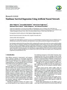
Figure 2

Figure 1

|

|

The recurrent architecture of Elman networks.

Cascade-correlation architecture.

contain a length of lagged values representing time hidden layer containing a single unit. The topology of a cascade-correlation network is depicted in Figure 1. As can be seen in Figure 1, the input units of a cascade-correlation ANN have direct connections with the output units, and as such the data are not forced through a layer of limiting sigmoidal functions. An indirect advantage of this is that there is no limit to the activation value obtained at the output layer. Using an appropriate output activation function can further ensure generalisation beyond the calibration range. As described in Imrie et al. (2000a), the cascadecorrelation algorithm employed in this paper has been subject to a number of alterations. One such adjustment was made to ensure that the network will generalise and the final model will perform adequately when confronted with fresh data. This ‘guidance system’ was developed according to the standard cross-verification procedure, whereby the available data are split into three parts: a training set used to adjust the weights, a testing set used to avoid over-training, and a separate verification set with which to judge the overall performance of the trained network.

series windows of the determinand of interest and other pertinent variables (e.g. Hsu et al. 1995; Minns & Hall 1997; Campolo et al. 1999; Zealand et al. 1999). However, when the forecast lead-time is greater than one time-step, it may be useful to use the ANN’s forecast of the modelled variable as an additional input to the next time step. This principle is used in recurrent neural networks, which were first conceived by Jordan (1986). These are now commonly employed on temporal processing tasks (Wang et al. 1996), although their application in hydrological modelling is not widely reported. The simplest form of recurrent ANN is the Elman network (Elman 1988), whose architecture is presented in Figure 2. These networks assume that that the ANN operates in discrete time steps. The activations of the hidden units at time t are fed backwards and used as inputs to ‘context units’ at time t + 1, representing a kind of shortterm memory. The importance and influence of these lag 1 inputs are determined during the training of the network. A recurrent version of the original cascade-correlation algorithm has also been developed (Fahlman 1991). In this case the hidden unit activations are no longer fed back to all of the other hidden units. Instead, every hidden unit has only one self-recurrent link, which is trained along

3.2 Recurrent modified cascade-correlation algorithm The

majority

of

ANN

forecasting

applications

in

hydrology involve the construction of input patterns that

with the candidate unit’s other input weights to maximise the correlation. When the candidate unit is added to the active network as a hidden unit, the recurrent link is frozen along with all other links.

158

D. F. Lekkas et al.

|



|

03.3

|

2001

The majority of recurrent ANN algorithms were orig-

observed flow (prediction error), then corrective action

inally designed for tasks associated with temporal

should be taken in order to modify future forecasts in an

sequences, such as natural language processing and recog-

attempt to improve performance. However, effort spent

nising characters from Morse code (Fahlman 1991; Wang

implementing an updating method should not be at the

et al. 1996). As such, the hidden unit activations are

expense of effort spent improving the model or quality of

recycled as internal state variables, and the resulting

input data, since the quality of the forecast model has the

ANNs are used to map sequences of inputs into desired

greatest impact on forecast accuracy (Bell & Moore 1998).

corresponding sequences of outputs. The problem posed

It should also be noted that improvements resulting

in river flow forecasting differs in that the aim is to provide

from updating reduce with the forecast lead-time since all

a continuous sequence of forecasts with lead times of

techniques rely upon the presence of persistence in the

greater than one time step. For this reason, the recurrent

prediction errors (Lees 2000a).

modified cascade-correlation algorithm developed in this paper recycles the output of the network instead of the activations of the hidden units. There are a number of advantages to this simple implementation: the number of input units does not grow as the hidden units are added; and it would be possible to directly determine the relative importance of the recycled values in a sensitivity analysis. It should be noted that there are also a number of possible drawbacks to the use of recurrent ANNs. Firstly, the procedure of training the weights in recurrent neural networks is much less orderly than in simple feedforward networks (Russell and Norvig 1995). The networks can become unstable and chaotic. In particular, for an ANN that uses its outputs as additional inputs on the next pattern, each input pattern will change after each weight update. This constitutes a moving target problem, as the error surface is continually changing as training proceeds. Furthermore, the benefits of recycling the output predictions will ultimately depend on the quality of the predictions themselves. However, results obtained in previous research showed that the recurrent version performed better in various river flow prediction applications than the modified cascade-correlation algorithm alone (Imrie 2000a), and so this algorithm will be used for the modelling undertaken in this paper.

4.1 Error prediction One way of developing an error prediction updating method is to represent the error fluctuation by an AutoRegressive Moving Average (ARMA) noise model (e.g. Ahsan & O’Connor 1994). This technique takes advantage of the dependence of model errors by characterising this dependence through a weighted combination of past prediction errors. The sequence of errors et can be simulated as et =

where

e

p t−p

+ at + O1at − 1 + . . . +

1

,

2

, . . .,

p

are the auto-regressive and O1, . . ., Oq

process with zero mean and variance s2a. The order of the ARMA model can be determined by examining autocorrelation (ACF) and the partial auto-correlation (PACF) functions of a prediction error time series generated from historical data. Once the structure has been determined then least squares (LS) is used to estimate the parameters. The error forecast et + f/t at the (t + f)th sampling instant is then given by

e

the performance of a real-time forecasting system is called

+...+

(8)

e

1 t − 1 + f/t

p t − p + f/t

Utilisation of the latest available observed data to improve

e

2 t−2

are the moving average parameters, and at is a random

et + f/t =

4 REAL-TIME ERROR UPDATING (EU)

+

e

1 t−1

Oqat − q

+...+

+ at + O1at − 1 + f/t + . . . + Oqat − q + f/t

and the updated flow forecast yut + f/t at time t + f by: yut + f/t = yt + f/t + et + f/t

updating. If an operational flow forecasting model produces forecasts that consistently do not agree with the

(9)

where yt + f/t is the f step ahead model flow forecast.

(10)

159

D. F. Lekkas et al.

|



|

03.3

|

2001

In contrast to state adjustment schemes, which internally adjust values within the model, the error prediction scheme is fully external to the deterministic operation. The result is a prediction of the future errors, which is added to the model simulation forecasts to form updated forecasts for different lead times. This means that the method can be used regardless of the type of forecast model, and can therefore also be applied to ANN forecasts. Error prediction is useful when the source of the error of the current event is unknown or untraceable and it performs slightly better in catchments with a slow response (Refsgaard 1997). However, one restriction associated with using error prediction is that, as the corrections are made by the difference between the simulated and the observed values of the flow, the flow data have to

Figure 3

|

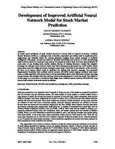
Map of River Trent catchment showing position of gauging stations.

be reliable (Lundberg 1982).

4.2 ANN error updating The recurrent modified cascade-correlation algorithm described above allows the most recent ANN forecasts to be utilised as inputs in the subsequent forecast. The use of this method necessitates that the patterns presented to the network are temporally consecutive. One potential improvement to this algorithm is to also include the most recent error calculated between the observed and predicted values. This procedure was implemented into the recurrent modified cascade-correlation algorithm, and its benefits are assessed in the subsequent case study. It is important to note that the error input must have an associated lag time that matches the length of the forecast. This constitutes an intrinsic form of the real-time updating techniques that were discussed in the previous section.

The aim was to create models that could forecast the flow at Colwick with a lead time of 12 hours. The size of the catchment upstream of Colwick is 7486 km2. Drought prevailed over this area during the years of 1995 and 1996 (Smith & Crymble 1998), and so flows during this period were generally low. Although 1997 saw a greater number of high flow events, the highest and most numerous flood peaks were observed in 1998. Therefore, in order to test the performance of the methods for significantly higher flows than those present in the calibration period, it was most informative to use the years 1996 and 1997 as calibration data, and to validate the models using data from 1998. The Colwick flow time series for all three years, showing the division of the data into calibration and verification datasets, is shown in Figure 4. A correlation analysis was performed on the data to identify suitable lags to be applied to each upstream gauging station time series in order to form the ANN’s input patterns and to define an appropriate range of TF model

5 RIVER FLOW PREDICTION

structures to be investigated. The intention was to provide the models with a snapshot of the current (t = 0 hours) and

River flow data covering the years 1996, 1997 and 1998

antecedent (t = − 1, − 2, . . . − n hours) conditions at each

were obtained from the Environment Agency of England

of the selected gauging stations, which could then be used

and Wales for a number of gauging stations located within

to predict the flow at Colwick at t = 12 hours. For Hopwas

the catchment of the River Trent, as shown in Figure 3.

Bridge and Izaac Walton, lags up to t = − 14 hours were

160

D. F. Lekkas et al.

|



Table 1

600

|

|

03.3

|

2001

Flow forecast results at Colwick with a lead time of 12 h

Calibration period

R2 (Verification)

Verification period

Testing period

500

Discharge (m3 / s)

400

Model

Original

With EU

300

ARMA

0.787

0.944

200

INL-TF

0.922

0.952

100

BP-ANN

0.907

0.966

RMCC-ANN

0.961

0.975

0 1/1/96

Figure 4

|

1/1/97

Date

1/1/98

31/12/98

Discharge data record for Colwick gauging station. INL-TF: Transfer Function models with Input Non-Linearity; EU: Error Updating; BP-ANN: Backpropagation ANN; RMCC-ANN: Recurrent Modified Cascade-Correlation ANN.

considered appropriate, whereas at Littlethorpe, which is closer to Colwick, lags up to t = − 12 hours were used. Two ANN models were developed, based upon the input data described above. All the ANNs incorporated linear activation functions at the output layer. The first

6 RESULTS AND DISCUSSION The overall performance of each model obtained was judged with respect to the verification data on the basis of the coefficient of efficiency, R2, defined as follows:

type was a traditional feed-forward backpropagation ANN trained with the gradient descent method, as described by Imrie et al. (2000a). The model was developed using the SNNS software package (Zell et al. 1995), the successful use of which has been reported in a number of appli-

where yp, and dp are the model predictions and target

cations (Abrahart & Kneale 1997; See & Openshaw 1998;

values for each pattern (sample) p respectively, and d z is

Tchaban et al. 1998; Campolo et al. 1999). The back-

the mean target output. The R2 coefficient is a useful

propagation ANN (BP-ANN) had one layer of 15 hidden

statistic in that it provides a measure of the proportion of

units. The error prediction technique discussed above

variance that is explained by the model. The closer its

was then applied to this model to assess the benefits of

value is to unity, the better the fit of the model.

real-time error updating.

The results obtained using each of the forecasting

The second type of ANN, the recurrent modified

methods over the verification period are presented in

cascade-correlation ANN (RMCC-ANN), was found to

Table 1. It can be seen that the simple ARMA method,

perform best when it included one recurrent output, that

which assumes linearity, provides the poorest predictions

is, the forecast representing time t + 11 was appended to

of all the models. In comparison with the linear ARMA

the input pattern for forecasting the flow at time t + 12.

model the non-linear TF method (INL-TF) provides con-

The ANN error updating method was then applied in

siderably better flow forecasts, suggesting that a non-

conjunction with this configuration.

linear method is required to provide a reasonable flow

Two types of time series models were developed: a

prediction model. The predictions made by each model

simple ARMA model and an INL-TF; all with a single a

can be compared in Figure 5. An inspection of the graph

and a single b parameter and a 12 hour lag. The error

shows that the non-linear model is superior to the ARMA

prediction technique was also utilised for real-time

model in terms of both the timing and magnitude of the

correction purposes.

peaks.

161

D. F. Lekkas et al.

|



|

03.3

|

2001

550 flow

flow

INL-TF

500

500

ARMA ARMA+EU

450

450

400

400

350

350

Discharge m3/s

Discharge m3/s

ARMA

300 250 200

300 250 200

150

150 100

100 24/10/98

26/10/98

28/10/98

30/11/98

1/11/98

3/11/98

5/11/98

50 24/10/98

Date

Figure 5

|

26/10/98

28/10/98

30/11/98

1/11/98

3/11/98

5/11/98

Date

Comparison between ARMA and INL-TF model. Figure 7

|

Comparison between original ARMA model and ARMA model with error updating.

flow BP-ANN

500

Discharge m3/s

RMCC-ANN

450

conjunction with each of the modelling techniques. The

400

application of EU resulted in an improvement in the

350

performance of each model. The most significant improve-

300

ment is observed when the method is applied to the

250

ARMA model, increasing the R2 from 0.787 to 0.944. Figure 7 compares the original ARMA forecasts with those

200

obtained when the error updating technique is applied. It

150

can be seen from this graph that the updating procedure

100

has allowed higher flows to be predicted, since it has been 22/10/98

24/10/98

26/10/98

28/10/98

30/11/98

1/11/98

3/11/98

5/11/98

Date

Figure 6

|

Comparison between Recurrent Modified Cascade-Correlation ANN and Backpropagation ANN.

able to compensate for the consistent underestimation of the original ARMA model. However, it can also be seen that the error updating technique has not improved the timing of the flow fluctuations. The changes observed when error updating is used with the INL-TF and BP-ANN models are less significant,

The BP-ANN, also non-linear, provides only slightly

but still constitute a sizeable improvement. The recurrent

better predictions than the INL-TF model. However, a

modified cascade-correlation algorithm is again improved

2

more significant increase in R was obtained using the

when the error updating method is introduced: however,

recurrent modified cascade correlation model. Figure 6

this increase from 0.961 to 0.975 is barely noteworthy. The

compares the predictions made by the BP-ANN with those

results obtained using the ILN-TF and the RMCC-ANN in

of the RMCC-ANN over a section of the verification

conjunction with their real-time error updating tech-

period. It can be clearly seen that the RMCC-ANN model

niques are plotted in Figure 8. The graph confirms that,

is far better able to capture the peak flow values than the

although the RMCC-ANN matches the observed flow

traditional BP-ANN.

slightly better than the INL-TF model, there is little differ-

The second column in Table 1 lists the R2 coefficients

ence in performance between the two models. While both

obtained when an error updating method is applied in

models perform very well, the minor fluctuations in the

162

D. F. Lekkas et al.

|



Flow INLTF+EU RMCC+EU

450

|

2001

strated in this paper, their application was limited to a single case study. It would therefore be inappropriate to draw firm conclusions about their overall performance.

400

Discharge m3/s

03.3

While the power of these techniques has been demon-

550 500

|

Additional case studies should be considered, using different catchment sizes and climates, to further assess their

350

overall performance.

300 250 200 150

ACKNOWLEDGEMENTS

100

The Environment Agency of England and Wales supplied

50 24/10/98

26/10/98

28/10/98

30/11/98

1/11/98

3/11/98

5/11/98

Date Figure 8

|

Comparison between INL-TF and RMCC-ANN, both with real-time error updating.

predicted flow series may indicate that the non-linearity of the two types of model has compromised their overall stability.

the data used in this paper. The funding for this research was provided by the UK Engineering and Physical Sciences

Research

pare the performance of two state-of-the-art data-based flow forecasting methodologies using real data from the

and

by

the

European

ABBREVIATIONS ANN ARMA BP-ANN EU INL-TF

Artificial Neural Network Auto-Regressive Moving Average Backpropagation ANN Error Updating Transfer Function models with Input Non-

RMCC-ANN

Linearity Recurrent Modified Cascade-Correlation

TF

ANN Transfer Function

7 CONCLUSIONS The objective of the paper was to demonstrate and com-

Council

Commission.

River Trent. The result of this comparison was that both the non-linear Transfer Function and Backpropagation ANN methods performed significantly better than the linear ARMA method, with little difference in performance. The best overall performance was obtained using the recurrent modified cascade-correlation ANN. The realtime updating techniques that were subsequently applied improved the forecast accuracy, particularly for the poorer models, showing that updating is a very important component of a real-time flood forecasting system. However, it was also noted that the application of the error updating method to the linear model could only improve its performance in terms of the magnitude of the flow, and not the timing of the peaks.

REFERENCES Abrahart, R. J. & Kneale, P. E. 1997 Exploring neural network rainfall-runoff modelling. BHS National Hydrology Symposium, Salford, UK, British Hydrological Society, pp 9.35–9.43. Ahsan, M. & O’Connor, K. M. 1994 A reappraisal of the Kalman filtering technique, as applied in river flow forecasting. J. Hydrol. 161, 197–226. Augusteijn, M. F. & Warrender, C. E. 1998 Wetland classification using optical and radar data and neural network classification. Int. J. Remote Sens. 19, 1545–1560. Bebis, G., Georgiopoulos, M. & Kasparis, T. 1997 Coupling weight elimination with genetic algorithms to reduce network size and preserve generalization. Neurocomputing 17, 167–194.

163

D. F. Lekkas et al.

|


Bell, V. A. & Moore, R. J. 1998 A grid-based distributed flood forecasting model for use with weather radar data: Part 2 Case studies. Hydrol. Earth Syst. Sci. 2, 283–298. Bishop, C. M. 1995 Neural Networks for Pattern Recognition. Clarendon Press, Oxford. Blanco, A., Delgado, M. and Pegalajar, M. C. 2000 A genetic algorithm to obtain the optimal neural network. Int. J. Approx. Reason. 23, 67–83. Campolo, M., Andreussi, P. & Soldati, A. 1999 River flood forecasting with a neural network model. Wat. Resources Res. 35, 1191–1197. Cluckie, I. 1993 Real-time hydrological forecasting. In Concise Encyclopaedia of Environmental Systems (ed. P. C. Young), pp. 291–298. Pergamon, Oxford. Cunge, J. A. 1969 On the subject of a flood propagation method. J. Hydraul. Res. IAHR 7, 205–230. Dawson, C. W. & Wilby, R. 1998 An artificial neural network approach to rainfall-runoff modelling. Hydrol. Sci. J. 43, 47–66. Dawson, C. W. & Wilby, R. L. 1999 A comparison of artificial neural networks used for river flow forecasting. Hydrol. Earth Syst. Sci. 3, 529–540. Durucan, S. & Imrie, C. E. 1998 The use of artificial neural networks in short-term river flow prediction. In Proceedings of the Fifth International Symposium on Environmental Issues and Waste Management in Energy and Mineral Production, Ankara, Turkey, Balkema, pp. 243–248. Elman, J. L. 1988 Finding structure in time. CRL Technical Report 8801, University of California at San Diego, Centre for Research in Language. Fahlman, S. E. 1988 An empirical study of learning speed in back-propagation networks. Carnegie Mellon University Technical Report CMU-CS-88-162. Fahlman, S. E. & Lebiere, C. 1990 The cascade-correlation learning architecture. Carnegie Mellon University Technical Report CMU-CS-90-100. Fahlman, S. E. 1991 The recurrent cascade-correlation architecture. Carnegie Mellon University Technical Report CMU-CS-91-100. Hecht-Nielsen, R. 1987a Counterpropagation networks. Appl. Opt. 26, 4979–4984. Hecht-Nielsen, R. 1987b Kolmogorov’s mapping neural network existence theorem. Proceedings of the 1st IEEE International Joint Conference on Neural Networks, San Diego, California, SOS Printing. Hirose, Y., Yamashita, K. & Hijayi, S. 1991 Back-propagation algorithm which varies the number of hidden units. Neural Networks 4, 61–66. Hopfield, J. J. 1987 Learning algorithms and probability distributions in feed-forward and feed-back networks. Proc. Nat. Acad. Sci., USA 84, 8429–8433. Hsu, K., Gupta, H. V. & Sorooshian, S. 1995. Artificial neural network modeling of rainfall-runoff process. Wat. Resources Res. 31(10), 2517–2530. Imrie, C. E. 2000 Artificial neural network modelling of river quality for short-term prediction of environmental impact. PhD thesis, Imperial College, London, UK.


|

03.3

|

2001

Imrie, C. E. & Durucan, S. 1999 River flow prediction using the cascade-correlation neural network learning architecture. In Proceedings of the Water 99 Joint Congress, Brisbane, Australia, Institute of Engineers Australia, pp. 94–99. Imrie, C. E., Durucan, S. & Korre, A. 2000a River flow prediction using artificial neural networks: generalisation beyond the calibration range. J. Hydrol. 233, 138–153. Imrie, C. E., Lekkas, D. F. & Lees M. J. 2000b. Comparison of non-linear transfer function and artificial network for flow routing. Proceedings of the British Hydrological Society 7th National Hydrology Symposium, Newcastle upon Tyne, UK, British Hydrological Society. pp. 5.15–5.16. Jordan, M. J. 1986 Attractor dynamics and parallelism in a connectionist sequential machine. In Proceedings of the Eighth Annual Conference of the Cognitive Science Society, pp. 531–546. Erlbaum, Hillsdale, NJ. Karnin, E. D. 1990 A simple procedure for pruning back-propagation trained neural networks. IEEE Trans. Neural Networks 1, 239–242. Karunanithi, N., Grenney, W. J., Whitley, D. & Bovee, K. 1994 Neural networks for river flow prediction. J. Comput. Civil Engng 8, 201–219. Kohonen, T. 1982 Self-organized formation of topologically correct feature maps. Biol. Cybern. 43, 59–69. Le Cun, Y., Denker, J. S. & Solla, S. A. 1990 Optimal brain damage. In Advances in Neural Information Processing Systems, (ed. D. S. Touretzky), vol. 2, pp. 598–605. Morgan Kaufmann, San Mateo, CA. Lees, M. J. et al. 1994 An adaptive flood warning scheme for the River Nith at Dumfries. In 2nd International Conference of River Flooding Hydraulics (ed. W. R. White & J. Watts), pp. 65–75, John Wiley & Sons, Chichester. Lees, M. J. 1997 Modelling and automatic control of flow regulation for multipurpose catchment management, BHS 6th National Hydrology Symposium. Institute of Hydrology, pp. 1.1–1.13. Lees, M. J. 2000a Data-based mechanistic modelling and forecasting of hydrological systems. J. Hydroinformatics 2(1), 15–34. Lees, M. J. 2000b Advances in transfer function based flood forecasting. In Flood Issues in Contemporary Water Management (ed. J. Marsalek), pp. 421–428. NATO Science Series 2/71. Kluwer, Dordrecht. Liong, S.-Y., Lim, W.-H. & Paudyal, G. N. 2000 River stage forecasting in Bangladesh: neural network approach. J. Comput. Civil Engng 14, 1–8. Lundberg, A. 1982 Combination of a conceptual model and an autoregressive error model for improving short time forecasting. Nord. Hydrol. 13, 233–246. Maier, H. R. & Dandy, G. C. 2000 Neural networks for the prediction and forecasting of water resources variables: a review of modelling issues and applications. Environ. Model. Software 15, 101–124. Miller, G. F., Todd, P. M. & Hegde, S. U. 1989 Designing neural networks using genetic algorithms. Proceedings of the Third International Conference on Genetic Algorithms and their Applications. Morgan Kaufmann, San Mateo, CA, pp. 379–384.

164

D. F. Lekkas et al.

|


Minns, A. W. & Hall, M. J. 1996 Artificial neural networks as rainfall-runoff models. J. Hydrol. Sci. 41, 399–417. Minns, A. W. & Hall, M. J. 1997 Living with the ultimate black box: more on artificial neural networks. BHS 6th National Hydrology Symposium, Salford, UK, British Hydrological Society, pp. 9.45–9.49. Muttiah, R. S., Srinivasan, R. & Allen, P. M. 1997 Prediction of two-year peak stream discharges using neural networks. J. Am. Water Resources Assoc. 33, 625–630. Powell, M. J. D. 1987 Radial basis functions for multivariable interpolation: a review. In Algorithms for Approximation (ed. J. C. Mason & M. G. Cox), pp. 143–167. Clarendon Press, Oxford. Reed, D. W. 1984 A review of British flood forecasting practice. Institute of Hydrology Report No. 90. Refsgaard, J. C. 1997 Validation and intercomparison of different updating procedures for real-time forecasting. Nord. Hydrol. 28, 65–84. Rumelhart, D. E., Hinton, E. & Williams, J. 1986 Learning internal representation by error propagation. Parallel Distributed Processing 1, 318–362. Russell, S. J. & Norvig, P. 1995 Artificial Intelligence: A Modern Approach. Prentice-Hall, Englewood Cliffs, NJ. See, L. Corne, S., Dougherty, M. & Openshaw, S. 1997 Some initial experiments with neural network models of flood forecasting on the River Ouse. Proceedings of the 2nd International Conference on GeoComputation, Dunedin, New Zealand, University of Otago, Dunedin, pp. 15–22.


|

03.3

|

2001

See, L. and Openshaw, S. 1998 Using soft computing techniques to enhance flood forecasting on the River Ouse. Proceedings of the 1998 Hydroinformatics Conference, Copenhagen, Denmark. Setiono, R. & Hui, L. C. K. 1995 Use of a quasi-Newton method in a feedforward neural-network construction algorithm. IEEE Trans. Neural Networks 6, 273–277. Smith, D. J. & Crymble, S. 1998 Water quality considerations in developing a new resource for water supply within the Midlands of England. Wat. Sci. Technol. 38(6), 201–208. Tchaban, T., Taylor, M. J. & Griffin, J. P. 1998 Establishing impacts of the inputs in a feedforward neural network. Neural Comput. Appl. 7, 309–317. Wang, D., Liu, X. & Ahalt, S. C. 1996 On temporal generalization of simple recurrent networks. Neural Networks 9, 1099–1118. Weigend, A. S., Rumelhart, D. E. & Huberman, B. A. 1990 Predicting the future: A connectionist approach. Int. J. Neural Syst. 1, 193–203. Yao, X. 1993 A review of evolutionary artificial neural networks. Int. J. Intell. Syst. 8, 539–567. Young, P. C. 1998 Data-based mechanistic modelling of environmental, ecological, economic and engineering systems. Environ. Model. Software 13, 105–122. Zealand, C. M., Burn, D. H. & Simonovic, S. P. 1999 Short term streamflow forecasting using artificial neural networks. J. Hydrol. 214, 32–48. Zell, A. et al. 1995 SNNS Version 4.1: User Manual. University of Stuttgart, Stuttgart, Germany.