Improved Particle Filtering Schemes for Target ... - Semantic Scholar

➠

➡ IMPROVED PARTICLE FILTERING SCHEMES FOR TARGET TRACKING Zhe Chen 1 , Thia Kirubarajan 1 , Mark R. Morelande 2 1. Communications Research Lab, McMaster University, Canada 2. Center for Sensor, Signal and Information Processing, University of Melbourne, Australia ABSTRACT In this paper, we propose two improved particle filtering schemes for target tracking, one based on gradient proposal and the other based on Turbo principle. We present the basic ideas and derivations and show detailed results of three tracking applications. Favorable experimental findings have shown the efficiency of our proposed schemes and their potential in other tracking scenarios. 1. INTRODUCTION Recent years have witnessed ever-growing efforts in applying particle filters to signal processing, communications, and machine learning [1]. Bearing the nature of recursive Bayesian estimation and sequential Monte Carlo sampling, particle filtering has demonstrated its potential in various nonlinear, non-Gaussian, non-stationary sequential estimation problems. Among many, target tracking problem provides a testbed for particle filter. As well known, the conventional Bayesian bootstrap [3] or SIR filtering (using prior proposal) has a drawback of ignoring the most recent observation. In this paper, we propose two improved particle filtering schemes to overcome this weakness and apply them in several tracking applications. The first improvement scheme is to use gradient information of the measurement model. The idea of gradient proposal is very heuristic, but it is very simple to implement and turns out to be quite efficient in practice [4]. We also propose another new particle filtering method based on Turbo principle (motivated from Turbo decoding in communications). Basically, we use one filter (so-called slave filter) to produce a first-stage (rough) estimate; and we run another filter (master filter) in parallel to yield the secondstage (ultimate) estimate, which uses its current as well as previous estimate for importance weights update in a recursive particle filtering fashion. The rest of the paper is organized as follows: In section 2, we briefly discuss the Bayesian bootstrap filter and then introduce the improved schemes for particle filtering. Section 3 is devoted to two simulated and one real-life tracking applications, followed by concluding remarks in Section 4. 2. PARTICLE FILTERING AND IMPROVED SCHEMES 2.1. State-Space Model and Bayesian Bootstrap Filter Consider a generic discrete-time nonlinear state space model: xn+1 yn

= =

f (n, xn , dn ), g(n, xn , vn ),

(1a) (1b)

where dn and vn characterize the dynamic and measurement noise processes, respectively. The state equation (1a) characterizes the

0-7803-8874-7/05/$20.00 ©2005 IEEE

state transition probability p(xn+1 |xn ), whereas the measurement equation (1b) describes the probability p(yn |xn ) which is further related to the measurement noise model. Simply say, particle filter uses a number of independent random variables called particles, sampled directly from the state space, to represent the posterior probability, and update the posterior by involving the new observations; the “particle system” is properly located, weighted, and propagated recursively according to the Bayesian rule. Specifically, using a sequential important sampling (SIS) scheme, it can be shown [2] that the importance weights update has the following recursive form: (i)

Wn(i) = Wn−1 (i)

(i)

(i)

(i)

p(yn |xn )p(xn |xn−1 ) (i)

(i)

q(xn |x0:n−1 , y0:n )

(i)

.

(2)

(i)

where Wn = p(xn )/q(xn ) denotes the importance weight, (i) (i) and q(xn |x0:n−1 , y0:n ) represents the proposal distribution. Choosing a proper proposal often has a crucial effect on the particle filtering performance. The well-known SIR and Bayesian bootstrap filter [3] use a transition prior as proposal, i.e. q(xn |xn−1 , y0:n ) = p(xn |xn−1 ); it then simplifies (2) to (i)

Wn(i) = Wn−1 p(yn |x(i) n ),

(3)

which essentially neglects the effect of recent observation yn . Despite its appealing simplicity, this proposal distribution is far from optimal and its resulted performance can be quite poor even a large number of particles are used. Many improved schemes (such as the auxiliary variable) have been developed in the literature [1]. In the following, we will describe two improved schemes in an attempt to efficiently incorporate the observation information into the sampling step. 2.2. Particle Filtering Using Gradient Proposal In order to use the recent observation, we propose to use the gradient information of (1b) to select the “informative” particles [4]. The main idea behind it is to introduce a MOVE-step to sampling for the proposal distribution, which is plugged in before the sampling step in the conventional SIR filter. This new algorithm essentially calculates the gradient information from the likelihood model and guides the particles towards the low-error region, along the gradient-descent direction; by assuming an additive measurement noise model in (1b), the MOVE-step is described by ˆ n|n−1 = x ˆ n−1|n−1 − η x

IV - 145


∂(yn − g(x))2


∂x x=ˆ x

(4) n−1|n−1

ICASSP 2005

➡

➡ slave filter

x n-1(i),W n-1(i)

iteration. Essentially, two filters are trying to solve the same filtering problem but looking at it from different perspectives; each one takes advantage of the result of the other at the previous step and thereby produces the solution in a cooperative way. Due to its similarity to Turbo decoding, we call the proposed filter structure as Turbo particle filter (TPF). In what follows, we will derive the update equation mathematically in detail. Let us write the filtering posterior in a slightly different way:

x n|n time n

time n+1

yn x n(i),W n(i)

master filter

p(xn |y0:n )

Fig. 1. A schematic diagram of Turbo particle filtering.

=

p(xn |yn , y0:n−1 ) p(yn |xn , y0:n−1 )p(xn |y0:n−1 ) p(yn |y0:n−1 ) p(yn |xn )p(xn |y0:n−1 ).

= where η ∈ [0.001, 0.01] is a small-valued step-size parameter. As expected from (4), the inclusion of current observation yn and the calculation of gradient information will tend to push the samples to a high-likelihood region, thereby providing more reliable predictive samples for the next step. In summary, the improved particle filtering with gradient proposal reads as follows: 1. For i = 1, · · · , Np , sample

(i) x0

∼ p(x0 ),

(i) W0

(i)

(i)

Wn(i) =

=

(8)

Np 

˜ (j) δ(xn−1 − x(j) ), W n−1 n−1

(9)

˜ where W n−1 are the normalized importance weights with the sum equal to unity. Hence, we can have  p(x(i) = p(x(i) n |y0:n−1 ) n |xn−1 )p(xn−1 |y0:n−1 )dxn−1 (j)

≈

A schematic diagram of Turbo particle filtering is illustrated in Fig. 1. In Fig. 1, there are two filters in parallel, to be run iteratively. The slave filter, being an extended Kalman filter (EKF) ˆ n|n , given the current here, is used to produce a rough estimate x (i) observation yn and previous state estimates xn−1 . This is done by the typical EKF equations. Note that in the prediction step, ev(i) ery particle xn−1 is passed through the state equation, where the predicted covariance can be estimated by the sample covariance, ˆ n|n−1 , or calculated through linearization; in the filtering step, P (i) instead of using all of the samples {ˆ xn|n−1 }, we only use its mean  (i)  ˆ n|n−1 = x ˆ n|n−1 , to perform the EKF update: value, x

Pn|n

,

j=1

2.3. Turbo Particle Filtering

ˆ n|n−1 + Kn (yn − g(ˆ x xn|n−1 )), ˆ ˆ Pn|n−1 + Kn Cn Pn|n−1 ,

(i)

q(xn |yn )

p(xn−1 |y0:n−1 ) ≈

(i) (i) xn−1|n−1 ) p(ˆ xn |ˆ (i) . Wn−1 p(yn |ˆ x(i) ) n (i) (i) p(ˆ xn |ˆ xn|n−1 )

ˆef f , if N ˆef f > Np /2, 5. Calculate effective sample size N resampling; otherwise go to Step 2.

=

(i)

(i)

4. Importance weights update:

ˆ n|n x

(i)

p(yn |xn )p(xn |y0:n−1 )

where q(xn |yn ) is the proposal distribution. Assuming that at time n, we have the simulated particles for approximating the posterior of time n − 1:

(i) ˆ (i) xn|n−1 ). 3. Importance sampling: x n ∼ p(xn |ˆ

=

(7)

Next, suppose we can draw samples {xn } from a proposal distribution, we need to find the importance ratios to appropriately weight the samples. Using the importance sampling trick, we have

= 1/Np .

2. For each sample {xn−1 }, update the sample via (4).

Wn(i)

∝

(5)

Np 

(j) ˜ (j) p(x(i) W n |xn−1 ). n−1

(10)

j=1

Substituting (10) into (8) yields the importance weights update: (i)

p(yn |xn ) Wn(i)

=

N p j=1

(j) ˜ (j) p(x(i) W n |xn−1 ) n−1

.

(i)

q(xn |yn )

(11)

Using the Gaussian approximation proposal (from the EKF), we (i) can draw samples {xn } from q = N (ˆ xn|n , Pn|n ), where Pn|n is obtained from (6). Now equation (11) naturally combines the prior and likelihood information, using previous weights and samples as well as observation yn . Finally, the master filter produces Np ˜ (i) (i) Wn xn . a (second-stage) mean estimate xn = i=1 In summary, a complete-step of TPF runs as follows:

(6)

ˆ n|n−1 CTn (Cn P ˆ n|n−1 CTn +Σv )−1 , and Cn is the where Kn = P linearized Jacobian matrix of the measurement equation, Pn|n is ˆ n|n the filtered state covariance. Note that the filtered estimate x ˆ n|n−1 , since it utiis more accurate than the predicted estimate x lizes the observation yn . In the meantime, the master filter, given (j) yn and the previous simulated samples {xn−1 }, as well as the ˆ n|n , runs a particle filtering procedure with a first-stage estimate x constructed suboptimal proposal distribution, and further produces (i) a second-stage posterior estimate xn . After a complete step, the master filter propagates its samples to the slave filter for the next

IV - 146

(j)

1. At time n, for j = 1, . . . , Np , given xn−1 (obtained from the master filter in the previous step) and yn , run the EKF updates (for the slave filter) to calculate the approximated Gaussian sufficient statistics (ˆ xn|n , Pn|n ).   (i) ˆ n|n , Pn|n . 2. Draw Np samples {xn } from N x 3. For the master filter, for i = 1, . . . , Np , calculate the im˜ n(i) }. portance weights via (11), and normalize them to get {W Np ˜ (i) (i) Wn xn . 4. Calculate the second-stage estimate: xn = i=1

ˆef f , if N ˆef f < Np /2, perform the resampling. 5. Calculate N 6. Copy the Np particles to the slave filter for the next step.

➡

➡ Ŧ3

1.2

x 10

SIR SIR+gradient

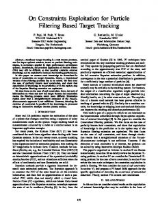
Table 1. Experimental results of bearing-only target tracking based on 50 Monte Carlo runs (excluding the divergence trials). filter MSE NMSE diver. rate EKF 0.0026 0.0168 0/50 UKF 0.0045 0.0232 0/50 SIR-prior (Np = 100) 0.0021 0.0150 3/50 SIR-gradient (Np = 100) 0.00014 0.0078 1/50 TPF-EKF (Np = 30) 0.00006 0.0009 0/50 TPF-UKF (Np = 30) 0.00006 0.0008 0/50

1

NMSE

0.8

0.6

0.4

0.2

0

Np

3. TRACKING APPLICATIONS

= =

500

Fig. 2. Performance (NMSE) comparison between the SIR and gradient proposal particle filters using varying numbers of particles, each based on 20 independent Monte Carlo runs.

Bearing-Only Tracking: First, we consider a bearing-only tracking benchmark problem [3]. Let (ν, νˆ, η, ηˆ) denote the x − y positions and velocities of a moving target. The state-space equations are described as follows: xn+1 yn

200

100

denote the state vector containing target position in x and y coordinate, target speed, heading, as well as turn rate. Under the SDE theory, the constant speed and turn rate (in the ideal CT model) will be instead modified as a Wiener process. Specifically, the 2nd-order Taylor approximation of the continuoustime state equation is described as [5]:

Fxn + Cdn , tan−1 (ηn /νn ) + vn ,

where xn = [νn , ν˙ n , ηn , ν˙ n ]T , dn = [d1,n , d2,n ]T , and ⎤ ⎤ ⎡ ⎡ 1 1 0 0 1 0 ⎢ 0 1 0 0 ⎥ ⎢ 1 0 ⎥ F=⎣ , C=⎣ . 0 0 1 1 ⎦ 0 1 ⎦ 0 0 0 1 0 1

xt = f (xτ ) + G(xτ )wt

2

The observation is a noisy bearing, and dn ∼ N (0, 0.001 I), vn ∼ N (0, 0.0052 ). The goal is to reconstruct the trajectory x0:n given the observed bearings y0:n and initial condition x0 = [−0.05, 0.001, 0.7, −0.055]T . The priors of particle filters are set up as p(x0 ) ∼ N (0, diag{0.052 , 0.0052 , 0.032 , 0.012 }) and Ep(x0 ) [x0 ] = [−0.06, 0.0015, 0.65, −0.05]T . Note that here the prior and likelihood are both peaked. The experimental comparisons are conducted between (i) EKF; (ii) unscented Kalman filter (UKF); (iii) SIR filter with a prior proposal; (iv) gradient proposal particle filter; (v) TPF with an EKF as slave filter; and (vi) TPF with a UKF as slave filter. A total of 50 Monte Carlo experiments with different random seeds are performed for each filtering scheme, using different number of particles. The error metrics of interest here are the mean-squared error (MSE), the normalized MSE (NMSE), as well as the divergence rate.1 Experimental results are summarized in Table 1. As seen, the two proposed particle filtering schemes outperform the conventional bootstrap filter. In this example, the TPF produces the best tracking result; but no big difference is observed between (v) and (vi), partially because the state equation is linear and Gaussian. Using the same number of particles, the gradient proposal obviously produces better results than the prior proposal; however, as expected, when Np gradually increases, the difference between them will be reduced; this has been confirmed in our experiments (see Fig. 2). Tracking with Coordinate Turn: Next, we consider a typical target tracking through a coordinated turn (CT), where the state-space model is described by a stochastic differential equation (SDE) and approximated by a 2nd-order weak Taylor approximation. See [5] for background and details. Let xt = [ξt , ςt , st , θt , ωt ]T

(12)

where δ = t − τ (we use δ = 1 in discretization), and ⎛ ξτ + δsτ cos(θτ ) − δ 2 sτ ωτ sin(θτ )/2 ⎜ ςτ + δsτ sin(θτ ) + δ 2 sτ ωτ sin(θτ )/2 ⎜ f (xτ ) = ⎜ sτ ⎝ θτ + δωτ ωτ G(xτ )

=

E(xτ )Vδ , ⎛

E(xτ )

=

Vδ

=

⎜ ⎜ ⎜ ⎝ 

⎞ ⎟ ⎟ ⎟, ⎠

with

σs cos(θτ ) 0 0 0 σs sin(θτ ) 0 0 0 0 0 σs 0 0 σω 0 0 0 0 0 σω   3 √ δ /3 √ 0 ⊗ I2×2 3δ/2 δ/2

⎞ ⎟ ⎟ ⎟, ⎠

where ⊗ denotes the Kronecker product; wt is a Wienner process approximated by standardized white Gaussian noise N (0, I4×4 ). The measurement equation consists of a “range-bearing” pair:  T yt = ξtt + ςt2 , tan−1 (ςt /ξt ) + vt (13) where the Gaussian measurement noise vt ∼ N (0, Σv ) is independent on the initial state and wt . The data trajectory was generated using the Euler approximation with sampling period of 1 second and 1000 intervals per sampling instant. Measurements are collected for 200 seconds with a constant sampling period. The noise and initial parameter setup in our experiment is as follows: σs2 = 1/5, σω2 = 5 × 10−7 , Σv = diag{100, (π/180)2 }, x0 ∼ N (µ0 , Σ0 ) with µ0 Σ0

1 By

divergence we mean the filter deviates from the target trajectory and is unable to come back to the true track.

IV - 147

= =

[1000, 2650, 150, π/2, −π/45]T , diag{400, 400, 25, (5π/180)2 , (0.2π/180)2 }.

➡

➠  ˆ 2 + |ς − ςˆ|2 performance comTable 2. The RMSE ≡ |ξ − ξ| parison (based on 20 Monte Carlo runs) with varying Np . Filter RMSE SIR-prior (Np = 500) 144.3 SIR-prior (Np = 1000) 91.6 SIR-prior (Np = 2000) 81.9 SIR-gradient (Np = 200) 142.3 SIR-gradient (Np = 500) 90.2 SIR-gradient (Np = 1000) 74.3 TPF-EKF (Np = 100) 158.7

xŦaxis

10000 5000 0

0

20

40

60

80

100

120

140

160

180

200

0

20

40

60

80

100

120

140

160

180

200

0

20

40

60

80

100

120

140

160

180

200

0

20

40

60

80

100

120

140

160

180

200

yŦaxis

5000

Target speed Target heading

0 200

20

150 100

0 Ŧ20

Turn rate

Ŧ0.06 Ŧ0.08 Ŧ0.1

0

20

40

60

80

100 Time step

120

140

160

180

200

Fig. 3. One typical result in tracking with CT experiment using gradient proposal particle filter (Np = 500, RMSE=87.5). Note that here the dynamic noise is peaked whereas the measurement noise is rather flat. Table 2 shows the comparison between the bootstrap filter (with prior proposal) and the SIR filter (with gradient proposal) and TPF, with varying number of particles. Fig. 3 shows one typical tracking result. MIMO Wireless Channel Tracking: Finally, we study a reallife MIMO wireless channel tracking problem (actually it is a channel/sybmol joint estimation problem but we ignore the symbol decoding part due to space limitation) [4]. The real-life wireless narrowband MIMO channel data were recorded in midtown Manhattan, New York city, January 2001. In particular, the state equation of the channel can be described by a first-order AR model driven by non-Gaussian noise (such as the mixture of Gaussians), whereas the measurement equation is described as [4]: #receivers

yj,n =



sk,n xjk,n + vj,n ,

k=1

where sk,n is the block of encoded symbols radiated by the kth transmitter at time n; xjk,n is the channel coefficient from the kth transmitter to the jth receiver at time n; yj,n is the signal observed at the input of the jth receiver; and vj,n is the measurement noise at the input of the jth receiver at time n, which is modeled by a Middleton Class A noise model. See [4] for more details. We have compared different trackers (including Kalman filter, mixture Kalman filters, and particle filters) [4], but here we only highlight the efficiency of the gradient proposal in this real-life application. As seen from Table 3, the proposed gradient proposal particle filter produces much better results (in terms of MSE as well as symbol error rate) than the conventional SIR filter, especially when using a small number particles. Namely, the particles drawn from the gradient proposal are more informative. This phenomenon has also been evidenced in the previous two applications. In terms of relative complexity and performance gain, compared to the Kalman filter (with complexity 1), the relative complexity factors of the SIR (with 100 particles) and our gradient SIR filters (with 20 particles) are 3.2 and 1.5, respectively; while their performance gains are 2.6 and 2.7, respectively! This huge gain is quite significant when complexity issue is concerned in industrial practice.

Table 3. The MSE of 2-by-2 MIMO wireless channel estimate and symbol error rate (SER) for various numbers of particles (at 10dB SNR) based on 100 Monte Carlo runs. Number of SIR-prior SIR-gradient Particles, Np MSE SER MSE SER 10 0.0615 0.0681 0.0233 0.0353 20 0.0431 0.0460 0.0206 0.0305 40 0.0338 0.0387 0.0196 0.0291 100 0.0257 0.0301 0.0188 0.0275 200 0.0227 0.0285 0.0183 0.0272

4. CONCLUDING REMARKS We have proposed two improved particle filtering schemes and demonstrated their potential merits in three tracking applications. In particular, the ad-hoc gradient proposal is quite efficient in various noise scenarios (esp. with small Σv ); whereas the TPF usually works well when variances Σd and Σv are both small (since the deterministic EKF gradually reduces the state-error variance). Eventually, the issue of performance and complexity tradeoff of particle filtering is central: choosing a better proposal distribution (with more computation per step) might ironically reduce the total complexity (in terms of required particle number simulation). In practice, we might design certain decision criteria for using different particle filters in different scenarios; in other words, we have to study the problem first and then choose a problem-specific filter. Acknowledgements: The authors thank Kris Huber for assistance in wireless channel tracking investigation. Z. C. was financially supported by a NSERC grant of Prof. Simon Haykin. 5. REFERENCES [1] A. Doucet, N. de Freitas, and N. Gordon, Eds. Sequential Monte Carlo Methods in Practice, Springer, 2001. [2] A. Doucet, S. Godsill, and C. Andrieu, “On sequential Monte Carlo sampling methods for Bayesian filtering,” Statist. Comput., vol. 10, pp. 197–208, 2000. [3] N. Gordon, D. Salmond, and A. F. M. Smith, “Novel approach to nonlinear/non-gaussian Bayesian state estimation,” IEE Proc.-F, vol. 140, pp. 107–113, 1993. [4] S. Haykin, K. Huber, and Z. Chen, “Bayesian sequential state estimation for MIMO wireless communication,” Proc. IEEE, vol. 92, no. 3, pp. 439–454, March 2004. [5] M. R. Morelande and N. J. Gordon, “Target tracking through a coordinated turn,” manuscript submitted to ICASSP2005.

IV - 148