Hindawi Publishing Corporation BioMed Research International Volume 2015, Article ID 960108, 12 pages http://dx.doi.org/10.1155/2015/960108
Research Article Improved Pre-miRNA Classification by Reducing the Effect of Class Imbalance Yingli Zhong,1 Ping Xuan,1 Ke Han,2 Weiping Zhang,1 and Jianzhong Li1 1
School of Computer Science and Technology, Key Laboratory of Database and Parallel Computing of Heilongjiang Province, Heilongjiang University, Harbin 150080, China 2 School of Computer and Information Engineering, Harbin University of Commerce, Harbin 150028, China Correspondence should be addressed to Weiping Zhang; zhangweiping
[email protected] and Jianzhong Li;
[email protected] Received 15 May 2015; Revised 18 October 2015; Accepted 20 October 2015 Academic Editor: Graziano Pesole Copyright © 2015 Yingli Zhong et al. This is an open access article distributed under the Creative Commons Attribution License, which permits unrestricted use, distribution, and reproduction in any medium, provided the original work is properly cited. MicroRNAs (miRNAs) play important roles in the diverse biological processes of animals and plants. Although the prediction methods based on machine learning can identify nonhomologous and species-specific miRNAs, they suffered from severe class imbalance on real and pseudo pre-miRNAs. We propose a pre-miRNA classification method based on cost-sensitive ensemble learning and refer to it as MiRNAClassify. Through a series of iterations, the information of all the positive and negative samples is completely exploited. In each iteration, a new classification instance is trained by the equal number of positive and negative samples. In this way, the negative effect of class imbalance is efficiently relieved. The new instance primarily focuses on those samples that are easy to be misclassified. In addition, the positive samples are assigned higher cost weight than the negative samples. MiRNAClassify is compared with several state-of-the-art methods and some well-known classification models by testing the datasets about human, animal, and plant. The result of cross validation indicates that MiRNAClassify significantly outperforms other methods and models. In addition, the newly added pre-miRNAs are used to further evaluate the ability of these methods to discover novel pre-miRNAs. MiRNAClassify still achieves consistently superior performance and can discover more pre-miRNAs.
1. Introduction MicroRNAs (miRNAs) are a set of short noncoding RNAs (∼22 nt) which bind with the mRNAs to regulate their expression and result in their cleavage or translational repression [1, 2]. The miRNAs usually participate in plenty of biological processes of animals and plants, including the developmental process, hematopoietic process, organogenesis, cell apoptosis, and cell proliferation in animals as well as growth and signal transduction in plants [3, 4]. An effective route for identifying miRNA is to predict the candidates by using computational methods, following by purposeful validation with the biological experiments. For the computational prediction of miRNAs, the methods based on homologous search, comparative genomics, and machine learning are three major categories. Although the first two kinds of methods can accurately identify miRNAs, they cannot identify those nonhomologous and speciesspecific miRNAs. The main reason is that they depend on
sequence homology and sequence conservation among the multiple species. The prediction based on machine learning is a de novo method which can identify nonhomologous and species-specific miRNAs. A prediction method based on machine learning uses real pre-miRNAs and pseudo premiRNAs as positive samples and negative samples, respectively. Many features are extracted from these samples according to the sequence and structure characteristics of premiRNAs. At last, a classification model is trained by using the samples and their features. So far, researchers have established models based on naive Bayes [5, 6], support vector machine (SVM) [7–9], Random Forest [10], and probabilistic colearning [11] and used these models to discriminate whether a given new sequence is a real pre-miRNA. Those sequences classified as real pre-miRNAs can be regarded as candidates. The position prediction method [12–14] is used to further determine the locations of miRNAs in the candidates. All pre-miRNA candidates and the location information of their miRNAs contribute to the subsequent biological validation.
2 When constructing a classification model, the experimental validated pre-miRNAs (real pre-miRNAs) are used as positive samples. As nearly all reported miRNAs located in the untranslated regions or intergenic regions, the sequences with stem-loop structure (pseudo pre-miRNAs) are collected from the protein-coding regions. These pseudo pre-miRNAs are regarded as negative samples. In reality, the number of negative samples is far greater than positive samples, which forms the severe class imbalance problem. It is well studied that a classification model trained with these samples would tend to determine a new sequence as a pseudo pre-miRNA (the majority class) [15]. Simultaneously, it would result in poor classification with respect to the minority class (real premiRNAs). Recently, several pre-miRNA classification methods have taken the imbalance problem into account. Triple-SVM [8] adopted random undersampling method to select the same number of negative samples with that of positive samples. PlantMiRNAPred [16] clustered the positive and negative samples according to their distribution. The equal number of representative positive and negative samples was selected as the training data. HuntMi [17] selected the partial negative samples based on the ROC score. Actually, there are a lot of various pseudo pre-miRNAs (negative samples) in the genomes. However, the methods with undersampling strategies ignored so much information of negative samples that the classification model has poor discriminative ability on them. In addition, miRNApre [18] only extracted the negative samples which are similar to the positive samples. As a result, the corresponding classification model has low robustness especially for the new pre-miRNAs that are not similar to the previous pre-miRNAs. Furthermore, this method also suffered from the negative effect of ignoring plenty of negative samples. On the other hand, microPred [19] generated the simulative positive samples based on SMOTE [20] to balance the numbers of positive and negative samples. Nonetheless, the process of generating simulative samples introduced the noisy data, which decrease the classification accuracy especially for positive samples. Therefore, it is essential to develop a new method to efficiently classify the imbalanced real and pseudo pre-miRNAs. In addition, the correct classification of real pre-miRNAs (positive samples) has greater value than the correct classification of pseudo pre-miRNAs (negative samples). It is helpful for the biologists to discover more novel pre-miRNAs. Hence a better classification model should provide a higher discrimination ability on the positive samples. In order to construct this type of model, cost-sensitive and ensemble learning [21, 22] has taken the various misclassification costs of different categories of samples and the class imbalance into account and achieved superior performance. Therefore, we proposed a classification method based on cost-sensitive and ensemble learning, which completely exploits the class imbalance factor and the cost factor of different categories. Through a series of iterations, the samples that are easy to be classified correctly and those that are easy to be misclassified are determined gradually and are assigned different weights. During each iteration, a new classification instance is trained by using the equal numbers of positive and negative samples.
BioMed Research International The weights of samples are updated according to the classification result of the new instance. After the iteration process is finished, all the instances are integrated into an ensemble classifier. First, each classification instance is trained by the same amount of positive and negative samples, which can efficiently relieve the negative effect of class imbalance. Second, the cost of misclassifying a positive sample is set higher than misclassifying a negative one. In this way, the classification accuracy on the positive samples is further improved. Third, the information of all the negative samples is exploited during the training process. At last, when a new classification instance is constructed, it focuses on the samples that are easy to be misclassified, which contributes to the improvement of the global classification performance. In addition, the data about human, animal, and plant were used to test our method, several state-of-the-art methods, and some classification models. Our method achieved superior classification performance not only for the cross validation but also for the testing on the newly added pre-miRNAs. The rest of this paper is organized as follows. Section 2 describes the features of real/pseudo pre-miRNAs and the process of constructing the ensemble classification model. In Section 3, we discuss the evaluation metrics of classification performance and compare and analyze the results of our method, other methods, and other classification models.
2. Methods 2.1. Features of Pre-miRNAs. It has been well studied that the pre-miRNAs have some characteristics about their sequences, secondary structures, and energy [23, 24]. The sequences and secondary structure of pre-miRNAs are usually conserved. The secondary structures often contain stem and loop regions. Furthermore, they have lower free energy. The previous pre-miRNA classification methods usually extracted different feature sets, as they focused on different characteristics of pre-miRNAs. So far, miPred [10], microPred [19], triplet-SVM [8], and miRNApre [18] have extracted the sequence-related, structure-related, and energy-related features. All the features are summarized as follows. First, there are 81 sequence-related features. (1) 16 features are related to the two adjacent nucleotides, and they represent the frequencies of two adjacent nucleotides, denoted as 𝑋𝑌%. 𝑋 and 𝑌 can be A (adenine), G (guanine), C (cytosine), or U (uracil). (2) The G + C% is used to describe the total content of G and C in the sequences. (3) 64 features are related to the frequencies of three adjacent nucleotides and denoted as 𝑋𝑌𝑍%, where 𝑋, 𝑌, and 𝑍 ∈ {A, G, C, U}. The following 49 features are related to the secondary structures of pre-miRNAs which can be obtained by using the structure-related prediction software such as the Vienna software package RNAfold [25]. (1) There are 8 features about the structure topology, including the structural diversity property Diversity, the structural frequency property Freq, the structural entropy-related properties dS and dS/L, the structural enthalpy-related properties dH and dH/L, the Shannon entropy value dQ, and the compactness of topology dF. (2) There are 9 features about base pairs, including
BioMed Research International the average amounts of base pairs |A − U|/𝐿, |G − C|/𝐿, and |G − U|/𝐿, the percentages of base pairs within the stem region |A − U|%/𝑛 stems, |G − C|%/𝑛 stems, and |G − U|%/𝑛 stems, the average number of base pairs in the stem region Avg BP Stem, the distance between a pair of bases dD, and the base-pairing tendency dP. (3) There are 32 features related to the characteristic of three adjacent nucleotides. “(” and “.” represent paired and unpaired bases, respectively. The nucleotide at the middle is recorded as A, G, C, or U. Thus, the percentages of the 32 combinations can be obtained. Finally, there are 9 features related to the energy of secondary structure: (1) the minimal free energy of the secondary structure dG, the minimal free energy-related features MFEI 1 , MFEI 2 , MFEI 3 , and MFEI 4 , and the overall free energy NEFE, the energy combination features 𝐷𝑖𝑓𝑓 = |𝑀𝐹𝐸 − 𝐸𝐹𝐸|/𝐿, and (2) the energy required for dissolving the secondary structure 𝑇𝑚 and 𝑇𝑚 /𝐿. These features have been successfully used to classify the real and pseudo pre-miRNAs. Therefore, the total of 139 features were merged to form our feature set. During the process of our feature extraction, the codes of miPred, microPred, triplet-SVM, and miRNApre were executed to obtain the respective features. All the extracted features were merged to represent each of real and pseudo pre-miRNAs. 2.2. Constructing the Cost-Sensitive Ensemble Model. A premiRNA classification method based on cost-sensitive ensemble learning is proposed and referred to as MiRNAClassify. We constructed multiple classification instances through a series of iterations and integrated these instances into an ensemble classifier. In this way, the information of all the positive and negative samples can be exploited. In the process of each iteration, a new classification instance is trained by the equal number of positive and negative samples, which can protect it from the negative effect of class imbalance. At the same time, each sample has its own weight which reflects the degree that it is easy to be misclassified. The training samples are selected in proportion to their weights, which make the new classification instance focus on the samples that are easy to be misclassified. Moreover, the weights of samples are adjusted according to the classification result of each instance. Hence when constructing a new instance, the new weight distribution of samples can be integrated to obtain a more accurate instance. In addition, as the cost of misclassifying each positive sample is higher than each negative sample, the positive samples are assigned greater cost weights. As shown in Figure 1, constructing the ensemble classification model includes the following 4 steps. (1) The sample set 𝑉 contains all the positive samples (real pre-miRNAs) and the negative samples (pseudo premiRNAs). 𝑛 is the number of the features. We extracted 𝑛 features from each positive sample and each negative one. Since the purpose of our cost-sensitive learning is to improve the discrimination ability on the positive samples (small class), the cost weights of positive samples should be set higher than those of negative samples. 𝐶𝑃 and 𝐶𝑁 represent the misclassification cost of positive and negative samples, respectively. The weight of each positive sample is initially set to 𝐶𝑃 /|𝑉| and that of each negative one is set to 𝐶𝑁/|𝑉|
3 where |𝑉| is the size of 𝑉. As 𝐶𝑃 should be higher than 𝐶𝑁, 𝐶𝑃 was set as 1 and 𝐶𝑁 varied from 0.1 to 0.9 with step length of 0.1. The best classification performance was achieved when 𝐶𝑃 = 1 and 𝐶𝑁 = 0.6. During the process of the first iteration, in the 𝑛dimensional sample space, the distance between any two of negative samples is calculated. Next, all the negative samples in 𝑉 are gathered into 𝑘 clusters based on 𝐾-means, and 𝑘 equals the number of positive samples. For each cluster, the negative sample that is closest to the center is obtained to be a training sample. Thus the initial training dataset 𝐴 1 is composed of 𝑘 positive samples and 𝑘 negative samples. The first classification instance based on the support vector machine (SVM) is trained by 𝐴 1 and denoted as 𝑀1 . The purpose of constructing 𝑀1 according to above steps is to quickly determine the positive and negative samples that are easy to be misclassified. As 𝑀1 is trained by the same number of positive and negative samples, 𝑀1 was not affected by the class imbalance. It has been confirmed that Rogers and Tanimoto measurement [26] could successfully measure the similarity between pre-miRNAs [16]. On the basis of the similarity measurement, the distance between two negative samples, such as 𝑥 and 𝑦, is defined as follows: dis (V𝑥 , V𝑦 ) = 1 −
V𝑥𝑡 ⋅ V𝑦 V𝑥𝑡 ⋅ V𝑥 + V𝑦𝑡 ⋅ V𝑦 − V𝑥𝑡 ⋅ V𝑦
,
(1)
where V𝑥 and V𝑦 are the feature vectors of 𝑥 and 𝑦, respectively, and V𝑥𝑡 and V𝑦𝑡 represent their transpose. (2) During the process of each subsequent iteration, the classification instance 𝑀𝑡 (1 ≤ 𝑡 ≤ 𝑇) classifies all the 𝑡 represents the global positive and negative samples in 𝑉. 𝐺𝑚 classification performance of 𝑀𝑡 and it is described in detail in Section 3.2. The weight of each positive and negative sample is adjusted according to the classification results of 𝑀𝑡 . The weight of a sample that was classified correctly is reduced and that of a sample that was misclassified remains unchanged. After a series of iterations were completed, a greater weight represents that a sample has been misclassified for more times. 𝑡 is 𝑀𝑡 ’s classification performance, the error rate of As 𝐺𝑚 𝑡 . 𝜃𝑡 is a parameter for adjusting the weight 𝑀𝑡 is 𝜑𝑡 = 1 − 𝐺𝑚 of each sample and 𝜃𝑡 = 𝜑𝑡 /(1 − 𝜑𝑡 ). Thus, the weight of the 1−|𝑝 (𝑥 )−𝑦 | 𝑖th sample 𝑥𝑖 at the 𝑡th iteration is updated as 𝑤𝑖𝑡−1 𝜃𝑡 𝑡 𝑖 𝑖 . 𝑡−1 Here, 𝑤𝑖 is the weight of 𝑥𝑖 at the (𝑡−1)th iteration, and 𝑦𝑖 is the true label of 𝑥𝑖 . If 𝑥𝑖 is a real pre-miRNA, 𝑦𝑖 is 1. Otherwise, 𝑥𝑖 is a pseudo pre-miRNA and 𝑦𝑖 is 0. 𝑝𝑡 (𝑥𝑖 ) represents the classification result of 𝑀𝑡 over 𝑥𝑖 , and 1 and 0 represent that 𝑥𝑖 is classified as positive sample and negative one, respectively. If 𝑥𝑖 is classified correctly, the value of 𝑝𝑡 (𝑥𝑖 ) is the same as its true label 𝑦𝑖 , we have |𝑝𝑡 (𝑥𝑖 ) − 𝑦𝑖 | = 0 and 1 − |𝑝𝑡 (𝑥𝑖 ) − 𝑦𝑖 | = 1. The weights of the correctly classified samples are multiplied by 𝜃𝑡 which is smaller than 1. Moreover, if the classification error rate is lower, the weights of the samples will become smaller. In terms of the misclassified samples, we have |𝑝𝑡 (𝑥𝑖 ) − 𝑦𝑖 | = 1 and 1 − |𝑝𝑡 (𝑥𝑖 ) − 𝑦𝑖 | = 0. Thus, their weights remain unchanged.
4
BioMed Research International
···
···
···
···
Extract n features and cluster the negative samples ···
···
···
···
···
Select the representative negative samples
Training dataset
Testing dataset ···
··· Construct a classification instance
···
···
···
Classify the samples and adjust their weights
M1
···
···
t=2
···
Select the negative samples
···
···
···
···
···
···
Classify the samples and adjust their weights M2
···
···
Select the negative samples
.. .
t=T
···
···
MT Construct the ensemble classifier
M1
M2
···
MT
Positive sample Negative sample
Figure 1: Constructing the integrated model to classify the real/pseudo pre-miRNAs.
(3) Assume the number of positive samples is 𝑘. To make the balance of positive and negative samples, we also selected 𝑘 negative samples. A negative sample with greater weight means that it has been misclassified for more times in the previous iterations. Therefore, we selected the negative samples in proportion to their weights. A new classification instance 𝑀𝑡+1 is trained by 𝑘 negative samples and 𝑘 positive
samples. At the same time, the weights of the training samples are integrated. (4) Steps (2) and (3) are repeatedly performed until the termination condition is satisfied. At last, 𝑇 classification instances are constructed and denoted as 𝑀1 , 𝑀2 , . . . , 𝑀𝑇 . The results of all instances are integrated based on the voting mechanism to give the
BioMed Research International
5
Input: a dataset, V, including all the positive and negative samples, and the negative samples are more than the positive samples. Output: ensemble classifier based on integrating multiple classification instances. (1) For 𝑖 = 1 to |𝑉| (2) If xi is a positive sample (3) 𝑤𝑖1 = 𝐶𝑃 /|𝑉|, 𝑤𝑖1 is the weight of 𝑥𝑖 (4) else (5) 𝑤𝑖1 = 𝐶𝑁 /|𝑉| (6) End If (7) End For (8) t is used to record the current iteration number, and its initial value is set as 1 (9) While (𝑡 ≤ 𝑇) (10) 𝐷𝑡 = Null, the negative training set 𝐷𝑡 is emptied (11) If 𝑡 equals 1 (12) All negative samples are gathered into k clusters based on the 𝐾-means method. Assume set P is composed of all the positive samples and the parameter 𝑘 = |𝑃| (13) For each cluster, the sample locating closest to the center is selected and added into 𝐷𝑡 . Furthermore, the number of negative samples |𝐷𝑡 | is equal to that of positive samples |𝑃| (14) else (15) According to the weights of negative samples, k negative samples are selected in proportion to their weights. These samples are added into 𝐷𝑡 and |𝐷𝑡 | = |𝑃| (16) End If (17) The training dataset is composed of 𝐷𝑡 and 𝑃. A new classification instance 𝑀𝑡 based on SVM is constructed by using the training dataset and integrating their weight distribution (18) 𝑀𝑡 is used to classify all the samples in 𝑉, evaluate its classification performance 𝐺𝑚 , and compute its classification error rate 𝜑𝑡 (19) The adjustment weight 𝜃𝑡 = 𝜑𝑡 /(1 − 𝜑𝑡 ) is calculated, and the weight of each positive and negative sample 1−|𝑝 (𝑥 )−𝑦 | is updated by using the rule 𝑤𝑖𝑡 = 𝑤𝑖𝑡−1 𝜃𝑡 𝑡 𝑖 𝑖 (20) 𝑡 = 𝑡 + 1 (21) End While (22) An integrated classifier is constructed by integrating 𝑇 classification instances based on the voting mechanism. The final classification result is obtained as follows. 𝑇 1 1 𝑇 1 { {1 if ∑ (log ) 𝑝𝑡 (𝑥) ≥ ∑log 𝑝𝑓 (𝑥) = { 𝜃 2 𝜃 𝑡 𝑡 𝑡=1 𝑡=1 { 0 otherwise { Algorithm 1: Algorithm of classifying the real/pseudo pre-miRNAs based on cost-sensitive ensemble learning.
final classification result. If the classification error rate 𝜑𝑡 is lower, 𝜃𝑡 is smaller and the determination weight log(1/𝜃𝑡 ) is greater. In this way, the result given by a instance with higher classification performance accounts for the greater proportion for the final result during the voting process. The algorithm of classification of the real/pseudo pre-miRNAs based on cost-sensitive ensemble learning is illustrated in Algorithm 1. The iterative process is terminated after the while loop is performed for 𝑇 times. When the value of 𝑇 is large enough, the error rate of the ensemble classifier can reach values as small as possible. In this study, the value of 𝑇 is set as 300.
3. Results and Discussion 3.1. Data Preparation. Both the sample set and the feature set are important factors influencing the pre-miRNA classification. Furthermore, the previous methods extracted various features because they focused on the different characteristics of pre-miRNAs. Therefore, in order to fairly compare with
each of previous methods, our classification method was also trained by the sample set and feature set which were the same as its ones. The information about the sample and feature of each compared method is listed as follows. MicroPred collected 691 real pre-miRNAs from the early version of miRNA database miRBase [27] (12.0 version, abbreviated as miRBase12.0) as the positive samples. The 660 pre-miRNAs have the stem-loop secondary structures and 31 pre-miRNAs have multiple stem-loops. These positive samples formed a positive dataset which is referred to as “MP positive set.” MicroPred obtained the 8494 pseudo hairpins as the negative samples and these hairpins were extracted from the human protein-coding regions. In addition, microPred collected 754 other types of noncoding RNAs, such as tRNA and rRNA, as the negative samples. The total 9248 negative samples formed a negative dataset named “MP negative set.” In terms of feature set, microPred obtained 21 features to train its classification model. PlantMiRNAPred was a classical method used to classify the plant pre-miRNAs. It collected the 2043 plant
6 pre-miRNAs in the miRBase14.0 as the positive samples and extracted the 2122 pseudo hairpins from the proteincoding regions of Arabidopsis thaliana and Glycine max as the negative samples. The positive samples and negative samples of PlantMiRNAPred formed its positive dataset “PMP positive set” and negative one “PMP negative set.” PlantMiRNAPred extracted 68 features from plant premiRNAs. HuntMi obtained 1406 human pre-miRNAs from miRBase17.0 and extracted 81228 human pseudo hairpins to form the human positive dataset “HM hsa positive set” and negative one “HM hsa negative set.” It also obtained 7053 real animal pre-miRNAs and 218154 animal pseudo hairpins to construct the animal positive dataset “HM animal positive set” and negative one “HM animal negative set,” respectively. In addition, it obtained 2172 plant pre-miRNAs and 114929 plant pseudo hairpins to form the plant positive dataset “HM plant positive set” and negative one “HM plant negative set.” HuntMi used 28 features to train its model. MiRNApre obtained 1496 human pre-miRNAs from miRBase17.0 as the positive samples and extracted 1446 pseudo hairpins similar with the positive samples. These pseudo hairpins are used as the negative samples. These positive samples and negative samples formed the positive and negative datasets “MP positive set” and “MP negative set.” MiRNApre extracted 98 features from each positive and negative sample. Moreover, the new pre-miRNAs about human, Arabidopsis lyrata, Oryza sativa, and Glycine max were reported by miRBase when our work was almost completed. These premiRNAs were also used to test the classification methods, which can further validate their ability of discovering the new pre-miRNAs. In addition, to compare our method with other methods simultaneously, all the positive and negative samples about human, animal, and plant were merged, respectively. The 1496 human pre-miRNAs and 81982 pseudo hairpins formed the human-related positive and negative datasets which are referred to as “Merged hsa positive set” and “Merged hsa negative set.” The animal-related positive and negative datasets contain 7053 real animal pre-miRNAs and 218154 pseudo hairpins and they are named “Merged animal positive set” and “Merged animal negative set.” The plantrelated datasets are “Merged plant positive set” and “Merged plant negative set” which are composed of 2172 plant real pre-miRNAs and 117051 pseudo hairpins. All the classification methods were tested by performing 5-fold cross validation on the three groups of datasets. The 355 new human premiRNAs (updated human dataset), 68 Arabidopsis thaliana pre-miRNAs (updated ath dataset), 169 Oryza sativa premiRNAs (updated osa dataset), and 302 Glycine max premiRNAs (updated gma dataset) were also used for testing. In terms of features, the 139 features described in Section 2.1 are used to represent each positive sample and negative one. 3.2. Performance Evaluation Metrics. Suppose that TP and TN represent the number of the correctly classified positive samples (real pre-miRNAs) and that of the correctly classified
BioMed Research International negative samples (pseudo pre-miRNAs), respectively. FP and FN represent the numbers of the misclassified positive and negative samples, respectively. Sensitivity (SE) represents the proportion of the positive samples that are classified successfully accounting for the total positive samples. Specificity (SP) represents the proportion of the successfully classified negative samples accounting for the total negative samples. Consider SE =
TP , TP + FN
TN SP = . TN + FP
(2)
For the pre-miRNA classification, if a classifier has higher SE and lower SP, it has poorer ability to identify the pseudo pre-miRNAs. Thus, many pseudo pre-miRNAs will be misclassified as the real pre-miRNAs, which reduces the possibility that the biological experiments can successfully identify pre-miRNAs. On the contrary, the classifier has poorer ability to identify the real pre-miRNAs, and many real pre-miRNAs will be misclassified as the pseudo pre-miRNAs, which reduces the possibility that the real pre-miRNAs are discovered by the experimental study. Therefore, the classifier should have both high SE and high SP. The global classification accuracy based on machine learning is usually evaluated by the parameter Acc. However, the number of pseudo pre-miRNAs is usually much greater than that of real pre-miRNAs, which causes TN and FP to be much higher than TP and FN. Then we have Acc =
TN TP + TN ≈ = SP. TP + TN + FP + FN TN + FP
(3)
Therefore, besides SE and SP, we also compute the geometric mean of SE and SP, denoted as 𝐺𝑚 , to evaluate the global classification performance: 𝐺𝑚 = √SE × SP.
(4)
3.3. Comparison with Other Methods and Classification Models. In order to compare MiRNAClassify with the stateof-the-art methods microPred [19], PlantMiRNAPred [16], HuntMi [17], and miRNApre [18], the 5-fold cross validation is performed. During the process of the cross validation, the positive and negative samples are randomly divided into 5 parts. 4 parts are used as the training samples, and the remaining part is used for testing. The testing dataset does not intersect with the training dataset. So it can objectively test the classification performances of the methods. Besides cross validation, the newly added human, animal, and plant pre-miRNAs are used to test the ability of discovering the new pre-miRNAs. MiRNAClassify is compared with other methods in two different ways. For one thing, in terms of each compared method, we choose its sample set and feature set to train MiRNAClassify. In this way, we compare MiRNAClassify with other methods, respectively. For another, MiRNAClassify is compared with all the other methods simultaneously by using the merged datasets and our feature set. In addition,
BioMed Research International
7
Table 1: Datasets and detailed classification results of MiRNAClassify and microPred. Species Homo sapiens
Dataset MP positive set MP negative set
Type Real Pseudo
Size 691 9248
MP updated set
Real
1186
100
100
90
90
80
80
70
70
60
60 (%)
(%)
Method MiRNAClassify microPred MiRNAClassify microPred
50
40
30
30
20
20
10
10 SE
SP
Gm
SE (hsa)
MiRNAClassify MicroPred
SP (%) 97.03 92.16
𝐺𝑚 (%) 96.71 91.40
50
40
0
SE (%) 96.40 90.65 90.56 85.16
0
SE
SP
Gm
SE (ath) SE (osa) SE (gma)
MiRNAClassify PlantMiRNAPred
Figure 2: Comparison of the performances of MiRNAClassify and microPred.
Figure 3: Comparison of the performances of MiRNAClassify and PlantMiRNAPred.
MiRNAClassify is compared with other classification models, including SVM, naive Bayes, and Random Forest.
PlantMiRNAPred. As shown in Figure 3 (details in Table 2), the first 3 columns are the comparison results of cross validation. MiRNAClassify achieved slightly better performance than PlantMiRNAPred. PlantMiRNAPred only extracted a small number of pseudo hairpins. The number of negative samples is close to that of positive samples, and there is no obvious class imbalance. It confirms that MiRNAClassify is still effective for this type of data. Actually, PlantMiRNAPred only selected partial positive and negative samples to train their model, which results in some of the sample information was lost. On the contrary, MiRNAClassify fully exploited the information from all the positive and negative samples by adjusting the sample weights and constructing multiple classification instances. In Figure 3, the last 3 columns are the results on 138 newly added Arabidopsis thaliana premiRNAs, 178 Oryza sativa pre-miRNAs, and 488 Glycine max pre-miRNAs. MiRNAClassify obtained consistently better classification accuracies. HuntMi was constructed to distinguish the real and pseudo pre-miRNAs about human, animal, and plant. The model of MiRNAClassify was also trained by using its samples and features. As Figure 4 shows (details in Table 3), MiRNAClassify and HuntMi performed the cross validation on three groups of datasets, respectively. It is obvious that the number of negative samples is far more than that of positive samples. There is a severe imbalance between the positive samples and negative samples. Although there are quite a lot of negative samples, HuntMi selected a small number of
3.3.1. Comparison Using the Same Dataset and Feature Set. MicroPred focused on classification of the human premiRNAs, and it generated new simulated positive samples based on SMOTE. In order to compare with microPred in a fair way, we used the sample set and feature set of microPred to train the model of MiRNAClassify. As shown in Figure 2 (details in Table 1), the first 3 columns are the results based on 5-fold cross validation, and the last column is the result for testing the newly added human pre-miRNAs. MicroPred obtained the lower sensitivity (SE = 90.65%) and specificity (SP = 92.16%) in the cross validation. The possible reason is that generating samples based on SMOTE introduced the noise data. MiRNAClassify is 5.31% better than microPred in overall accuracy 𝐺𝑚 . SE increased by 5.75% and SP increased by 4.87%. For the dataset that composed of 1186 newly added human pre-miRNAs, MP updated set, the SEs of MiRNAClassify and microPred are 90.56% and 85.16%, respectively. These SEs are not as good as those in the cross validation. The main reason is that MicroPred used the premiRNAs in the early version of miRBase and the new premiRNAs for testing are even more than the pre-miRNAs used to train its classification model. PlantMiRNAPred mainly studied the classification of plant pre-miRNAs. The model of MiRNAClassify was constructed by using the same sample and feature sets with
8
BioMed Research International Table 2: Datasets and detailed classification results of MiRNAClassify and PlantMiRNAPred.
Method MiRNAClassify PlantMiRNAPred MiRNAClassify PlantMiRNAPred MiRNAClassify PlantMiRNAPred MiRNAClassify PlantMiRNAPred
Species
Dataset PMP positive set PMP negative set
Type Real Pseudo
Size 2043 2122
Arabidopsis thaliana
PMP ath updated set
Real
138
Oryza sativa
PMP osa updated set
Real
178
Glycine max
PMP gma updated set
Real
488
Plant
SE (%) 96.57 95.10 92.75 90.58 77.53 67.42 90.78 86.07
SP (%) 98.35 97.17
𝐺𝑚 (%) 97.46 96.13
SP (%) 98.35 96.94 97.55 95.95 97.82 95.87
𝐺𝑚 (%) 97.75 95.98 96.64 95.03 95.54 93.77
Table 3: Datasets and detailed classification results of MiRNAClassify and HuntMi. Method MiRNAClassify HuntMi MiRNAClassify HuntMi MiRNAClassify HuntMi MiRNAClassify HuntMi MiRNAClassify HuntMi MiRNAClassify HuntMi MiRNAClassify HuntMi
Species
Dataset HM hsa positive set HM hsa negative set HM animal positive set HM animal negative set HM plant positive set HM plant negative set
Type Real Pseudo Real Pseudo Real Pseudo
Size 1406 81228 7053 218154 2172 114929
Homo sapiens
HM hsa updated set
Real
445
Arabidopsis thaliana
HM ath updated set
Real
68
Oryza sativa
HM osa updated set
Real
169
Glycine max
HM gma updated set
Real
302
Homo sapiens Animal Plant
100 90 80 70
(%)
60 50 40 30 20 10 0
SE
SP hsa
Gm
SE
SP Gm Animal
SE
SP Gm Plant
MiRNAClassify HuntMi
Figure 4: Comparison of the performances of MiRNAClassify and HuntMi based on 5-fold cross validation.
negative samples based on the ROC values to train its model. Apparently, it lost a large amount of information of negative samples. MiRNAClassify completely presented its advantage
SE (%) 97.15 95.02 95.74 94.11 93.32 91.71 93.93 92.14 92.65 91.18 75.74 69.82 92.72 88.41
in processing the class imbalance and achieved superior performance. In addition, we performed further testing using the newly added human, Arabidopsis thaliana, Oryza sativa, and Glycine max pre-miRNAs. The result was demonstrated in Figure 5, which confirms that MiRNAClassify can discover more new pre-miRNAs. We found that the classification performances of these two methods on newly added plant pre-miRNAs were worse than the performances on the new human pre-miRNAs. One of the important reasons is that the sequences and structures of plant pre-miRNAs are more complicated than those of human pre-miRNAs. Although miRNApre was tested on human, animal, and plant, only the training and testing samples about human could be obtained. Therefore, the human-related dataset was used to train the model of MiRNAClassify. Since miRNApre only selected the negative samples which are similar to the positive ones, the negative dataset is only composed of 1446 samples. The positive dataset contains 1496 samples (Table 4). There is no class imbalance because the number of positive samples nearly equals that of negative samples. In this case, the cross validation performance of MiRNAClassify is still better than miRNApre, as shown in the first 3 columns of Figure 6. In addition, we obtained 355 new human premiRNAs for further testing. The SEs of MiRNAClassify and miRNApre are 91.2% and 90.1%, respectively. The SEs are not
BioMed Research International
9
Table 4: Datasets and detailed classification results of MiRNAClassify and miRNApre. Method
Species
MiRNAClassify miRNApre
Homo sapiens
MiRNAClassify miRNApre
Dataset
Type
Size
SE (%)
SP (%)
𝐺𝑚 (%)
MP positive set MP negative set
Real Pseudo
1496 1446
98.33 97.66
98.27 97.23
98.29 97.44
MP updated set
Real
355
91.27 90.14
Table 5: The classification results of MiRNAClassify and other methods over the merged datasets and the updated datasets. Accuracy (%)
Method
Merged Merged human dataset animal dataset
Merged plant dataset
Updated Updated human dataset ath dataset
Updated Updated osa dataset gma dataset
MiRNAClassify
SE SP 𝐺𝑚
97.93 98.30 98.11
95.85 97.62 96.73
93.37 97.91 95.61
94.08
92.65
79.29
93.05
MicroPred
SE SP 𝐺𝑚
92.25 95.70 93.96
91.61 94.85 93.21
89.50 93.10 91.28
91.27
89.71
66.86
85.76
PlantMiRNAPred
SE SP 𝐺𝑚
93.58 91.20 92.38
92.70 88.60 90.63
91.39 87.10 89.22
92.11
89.71
70.42
88.41
HuntMi
SE SP 𝐺𝑚
95.32 97.11 96.21
94.14 96.07 95.10
91.76 95.94 93.83
92.68
91.18
72.78
89.07
miRNApre
SE SP 𝐺𝑚
97.39 90.90 94.09
93.49 89.80 91.63
91.71 88.10 89.89
90.14
89.71
71.01
86.09
100 90 80 70
(%)
60 50 40 30 20 10 0
SE (hsa)
SE (ath)
SE (osa)
SE (gma)
MiRNAClassify HuntMi
Figure 5: Comparison of the performances of MiRNAClassify and HuntMi on the newly added data.
as good as those obtained in the cross validation. The reason may be that the extracted negative samples were very similar to the positive samples which resulted in the low robustness of the classification models.
3.3.2. Comparison over the Merged Datasets. Besides comparison with each method, respectively, we tested MiRNAClassify and other methods simultaneously by using the merged datasets about human, animal, and plant and the newly updated datasets and extracting a set of same features. It is worth noting that the number of negative samples is much greater than that of positive samples in each merged dataset. The classification results are demonstrated in Table 5. MiRNAClassify performed the best not only over the merged datasets but also over the updated datasets. HuntMiRNA also achieved decent prediction performance. MicroPred, PlantMiRNAPred, and miRNApre obtained the inferior results, especially over the negative samples. In terms of MicroPred, more simulated positive samples have to be generated because there are so many negative samples, which also introduced more noisy data. The possible reason for the worse performance of PlantMiRNAPred and miRNApre is that most of information about negative samples was abandoned and their discriminative ability on negative samples was reduced greatly. In addition, a paired 𝑡-test was used to determine whether MiRNAClassify’s global performance (𝐺𝑚 ) over the 3 groups of merged datasets and its accuracy (SE) over the 4 updated datasets is higher than other methods. The corresponding 𝑝 values are listed in Table 6. The statistic results confirm that MiRNAClassify outperforms other methods significantly at the significance level 0.05.
10
BioMed Research International
Table 6: The statistic results obtained by using paired t-test over the prediction performance of MiRNAClassify and that of another method. Different datasets 𝑝 values on three groups of datasets 𝑝 values on four updated datasets
microPred
PlantMiRNAPred
HuntMi
miRNApre
0.0019 0.0339
4.9374𝑒 − 04 0.0284
9.7070𝑒 − 04 0.0354
0.0050 0.0108
100 90
Table 7: The classification results of MiRNAClassify and three classification models over the merged datasets.
80
Classification models
70
SVM SVM + SMOTE Naive Bayes Naive Bayes + SMOTE Random Forest Random Forest + SMOTE MiRNAClassify
(%)
60 50 40 30 20 10 0
SE
SP
Gm
SE (hsa)
MiRNAClassify miRNApre
Figure 6: Comparison of the performances of MiRNAClassify and miRNApre.
3.3.3. Comparison with Other Classification Models. We use 5-fold cross validation to compare MiRNAClassify with other well-known classification models including the standard SVM, naive Bayes, and Random Forest. These models under SMOTE method were further developed to compare with MiRNAClassify. All the models were trained by the merged datasets and the same set of features, and their classification results are demonstrated in Table 7. For the datasets with severe class imbalance, MiRNAClassify demonstrated its ability to process the imbalanced data and achieved the best performance. As expected, the standard classification models overlearned the information of majority class and obtained the small SEs and the great SPs. After the SMOTE method was applied to balance the positive and negative samples, these models except naive Bayes obtained decent improvement on 𝐺𝑚 values. The main reason is that naive Bayes has intrinsic resistance to the class imbalance. However, the classification models under SMOTE method, SVM, and Random Forest obtained nearly consistent performances which were slightly better than naive Bayes. It confirmed that SVM has the excellent generalization ability. In particular, each classification instance of MiRNAClassify was established based on SVM, which was one of the important factors that MiRNAClassify could perform well. After exerting 𝑡-test on the 𝐺𝑚 values obtained by MiRNAClassify and other models, the statistic results in Table 8 indicated that MiRNAClassify achieved significantly better performance.
SVM SVM + SMOTE Naive Bayes Naive Bayes + SMOTE Random Forest Random Forest + SMOTE MiRNAClassify SVM SVM + SMOTE Naive Bayes Naive Bayes + SMOTE Random Forest Random Forest + SMOTE MiRNAClassify
SE (%) Human 69.18 92.25 87.43 90.24 67.78 91.51 97.93 Animal 69.03 91.61 85.04 90.83 69.52 91.12 95.85 Plant 68.51 89.50 82.91 87.20 68.32 89.18 93.37
SP (%)
𝐺𝑚 (%)
99.83 95.70 96.12 94.43 99.82 95.34 98.30
83.11 93.96 91.67 92.31 82.26 93.41 98.11
98.14 94.85 95.03 92.61 98.72 95.01 97.62
82.31 93.21 89.90 91.71 82.84 93.05 96.73
99.24 93.10 96.75 92.61 99.35 92.87 97.91
82.45 91.28 89.57 89.86 82.39 91.01 95.61
4. Conclusions A new method based on cost-sensitive and ensemble learning (MiRNAClassify) was developed to classify the imbalanced real and pseudo pre-miRNAs. The multiple classification instances were constructed and integrated to classify a query sequence. Each instance was trained by the same number of positive and negative samples, which effectively relieved the negative effect of class imbalance. At the same time, the information of all the positive and negative samples was completely exploited. The weight of each sample embodied the possibility that it would be misclassified. Based on the sample weight, the new classification instance could focus on the samples that are easy to be misclassified. All of the above contribute to the more accurate classification performance. MiRNAClassify has been compared with the previous methods, microPred, PlantMiRNAPred, HuntMi, and miRNApre. Not only the human data but also the animal and
BioMed Research International
11
Table 8: The statistic results obtained by using paired t-test over the prediction performance of MiRNAClassify and that of another classification model. p value p value
SVM 7.3053𝑒 − 04 SVM + SMOTE 0.0019
plant data were used to test their performance. MiRNAClassify outperformed better than other methods during the cross validation and could discover more newly added premiRNAs. In addition, we compared MiRNAClassify with other methods and several well-known classification models by using the merged and imbalanced datasets. MiRNAClassify demonstrated its ability of processing the imbalance and achieved significantly better performance.
Conflict of Interests The authors declare that there is no conflict of interests regarding the publication of this paper.
Authors’ Contribution Yingli Zhong and Ping Xuan contributed equally to this work.
Acknowledgments The work was supported by the National Natural Science Foundation of China (61302139 and 61402138), China Postdoctora l Science Foundation (2014M550200 and 2014M561350), China Postdoctoral Science Special Foundation (2015T80367), the Natural Science Foundation of Heilongjiang Province (F201206, E201452, F2015013, and F201426), the Science and Research Foundation of Heilongjiang Education Department (12541606), the Postdoctoral Foundation of Heilongjiang Province (LBH-Z14152), the Support Program for Young Academic Key Teacher of Higher Education of Heilongjiang Province (1254G030), the Young Reserve Talents Research Foundation of Harbin Science and Technology Bureau (2015RQQXJ082 and 2015RAQXJ004), the Distinguished Youth Foundation of Heilongjiang University (JCL201405), and Key Laboratory Fund of Heilongjiang Province and Ministry of Education (Heilongjiang University).
References [1] D.P.Bartel, “MicroRNAs: genomics, biogenesis, mechanism, and function,” Cell, vol. 116, no. 2, pp. 281–297, 2004. [2] D. P. Bartel, “MicroRNAs: target recognition and regulatory functions,” Cell, vol. 136, no. 2, pp. 215–233, 2009. [3] S. L. Ameres and P. D. Zamore, “Diversifying microRNA sequence and function,” Nature Reviews Molecular Cell Biology, vol. 14, no. 8, pp. 475–488, 2013. [4] B.Zhang,X.Pan,G.P.Cobb,andT.A.Anderson,“Plant microRNA: a small regulatory molecule with big impact,” Developmental Biology, vol. 289, no. 1, pp. 3–16, 2006.
Naive Bayes 6.2651𝑒 − 04 Naive Bayes + SMOTE 0.0010
Random Forest 0.0015 Random Forest + SMOTE 0.0028
[5] M. Yousef, M. Nebozhyn, H. Shatkay, S. Kanterakis, L. C. Showe, and M. K. Showe, “Combining multi-species genomic data for microRNA identification using a Na¨ıve Bayes classifier,” Bioinformatics, vol. 22, no. 11, pp. 1325–1334, 2006. [6] M. Yousef, S. Jung, L. C. Showe, and M. K. Showe, “Learning from positive examples when the negative class is undetermined-microRNA gene identification,” Algorithms for Molecular Biology, vol. 3, article 2, 2008. [7] K. L. S. Ng and S. K. Mishra, “De novo SVM classification of precursor microRNAs from genomic pseudo hairpins using global and intrinsic folding measures,” Bioinformatics, vol. 23, no. 11, pp. 1321–1330, 2007. [8] C. Xue, F. Li, T. He, G.-P. Liu, Y. Li, and X. Zhang, “Classification of real and pseudo microRNA precursors using local structuresequence features and support vector machine,” BMC Bioinformatics, vol. 6, article 310, 2005. [9] J. Ding, S. Zhou, and J. Guan, “MiRenSVM: towards better prediction of microRNA precursors using an ensemble SVM classifier with multi-loop features,” BMC Bioinformatics, vol. 11, supplement 11, article S11, 2010. [10] P. Jiang, H. Wu, W. Wang, W. Ma, X. Sun, and Z. Lu, “MiPred: classification of real and pseudo microRNA precursors using random forest prediction model with combined features,” Nucleic Acids Research, vol. 35, no. 2, pp. W339–W344, 2007. [11] J.-W. Nam, K.-R. Shin, J. Han, Y. Lee, V. N. Kim, and B.-T. Zhang, “Human microRNA prediction through a probabilistic co-learning model of sequence and structure,” Nucleic Acids Research, vol. 33, no. 11, pp. 3570–3581, 2005. [12] P. Xuan, M. Guo, Y. Huang, W. Li, and Y. Huang, “Maturepred: efficient identification of microRNAs within novel plant premiRNAs,” PLoS ONE, vol. 6, no. 11, Article ID e27422, 2011. [13] M. Leclercq, A. B. Diallo, and M. Blanchette, “Computational prediction of the localization of microRNAs within their premiRNA,” Nucleic Acids Research, vol. 41, no. 15, pp. 7200–7211, 2013. [14] C. He, Y.-X. Li, G. Zhang et al., “MiRmat: mature microRNA sequence prediction,” PLoS ONE, vol. 7, no. 12, Article ID e51673, 2012. [15] G. M. Weiss, “Mining with rarity: a unifying framework,” ACM SIGKDD Explorations Newsletter, vol. 6, no. 1, pp. 7–19, 2004. [16] P. Xuan, M. Guo, X. Liu, Y. Huang, W. Li, and Y. Huang, “PlantMiRNAPred: efficient classification of real and pseudo plant pre-miRNAs,” Bioinformatics, vol. 27, no. 10, Article ID btr153, pp. 1368–1376, 2011. [17] A. Gudy´s, M. W. Szcze´sniak, M. Sikora, and I. Makałowska, “HuntMi: an efficient and taxon-specific approach in premiRNA identification,” BMC Bioinformatics, vol. 14, article 83, 2013. [18] L. Wei, M. Liao, Y. Gao, R. Ji, Z. He, and Q. Zou, “Improved and promising identification of human microRNAs by incorporating a high-quality negative set,” IEEE/ACM Transactions on Computational Biology and Bioinformatics, vol. 11, no. 1, pp. 192–201, 2014.
12 [19] R. Batuwita and V. Palade, “MicroPred: effective classification of pre-miRNAs for human miRNA gene prediction,” Bioinformatics, vol. 25, no. 8, pp. 989–995, 2009. [20] N. V. Chawla, K. W. Bowyer, L. O. Hall, and W. P. Kegelmeyer, “SMOTE: synthetic minority over-sampling technique,” Journal of Artificial Intelligence Research, vol. 16, no. 1, pp. 321–357, 2002. [21] Y. Sun, M. S. Kamel, A. K. C. Wong, and Y. Wang, “Costsensitive boosting for classification of imbalanced data,” Pattern Recognition, vol. 40, no. 12, pp. 3358–3378, 2007. [22] Y. Freund and R. E. Schapire, “A decision-theoretic generalization of on-line learning and an application to boosting,” Journal of Computer and System Sciences, vol. 55, no. 1, pp. 119–139, 1997. [23] P. Sætrom, O. Snøve Jr., M. Nedland et al., “Conserved microRNA characteristics in mammals,” Oligonucleotides, vol. 16, no. 2, pp. 115–144, 2006. [24] B. Zhang, X. Pan, C. H. Cannon, G. P. Cobb, and T. A. Anderson, “Conservation and divergence of plant microRNA genes,” The Plant Journal, vol. 46, no. 2, pp. 243–259, 2006. [25] I. L. Hofacker, B. Priwitzer, and P. F. Stadler, “Prediction of locally stable RNA secondary structures for genome-wide surveys,” Bioinformatics, vol. 20, no. 2, pp. 186–190, 2004. [26] D. J. Rogers and T. T. Tanimoto, “A computer program for classifying plants,” Science, vol. 132, no. 3434, pp. 1115–1118, 1960. [27] A. Kozomara and S. J. Griffiths, “MiRBase: annotating high confidence microRNAs using deep sequencing data,” Nucleic Acids Research, vol. 42, no. 1, pp. D68–D73, 2014.
BioMed Research International
International Journal of
Peptides
BioMed Research International Hindawi Publishing Corporation http://www.hindawi.com
Volume 2014
Advances in
Stem Cells International Hindawi Publishing Corporation http://www.hindawi.com
Volume 2014
Hindawi Publishing Corporation http://www.hindawi.com
Volume 2014
Virolog y Hindawi Publishing Corporation http://www.hindawi.com
International Journal of
Genomics
Volume 2014
Hindawi Publishing Corporation http://www.hindawi.com
Volume 2014
Journal of
Nucleic Acids
Zoology
International Journal of
Hindawi Publishing Corporation http://www.hindawi.com
Hindawi Publishing Corporation http://www.hindawi.com
Volume 2014
Volume 2014
Submit your manuscripts at http://www.hindawi.com The Scientific World Journal
Journal of
Signal Transduction Hindawi Publishing Corporation http://www.hindawi.com
Genetics Research International Hindawi Publishing Corporation http://www.hindawi.com
Volume 2014
Anatomy Research International Hindawi Publishing Corporation http://www.hindawi.com
Volume 2014
Enzyme Research
Archaea Hindawi Publishing Corporation http://www.hindawi.com
Hindawi Publishing Corporation http://www.hindawi.com
Volume 2014
Volume 2014
Hindawi Publishing Corporation http://www.hindawi.com
Biochemistry Research International
International Journal of
Microbiology Hindawi Publishing Corporation http://www.hindawi.com
Volume 2014
International Journal of
Evolutionary Biology Volume 2014
Hindawi Publishing Corporation http://www.hindawi.com
Volume 2014
Hindawi Publishing Corporation http://www.hindawi.com
Volume 2014
Molecular Biology International Hindawi Publishing Corporation http://www.hindawi.com
Volume 2014
Advances in
Bioinformatics Hindawi Publishing Corporation http://www.hindawi.com
Volume 2014
Journal of
Marine Biology Volume 2014
Hindawi Publishing Corporation http://www.hindawi.com
Volume 2014