when a sufficiently large number of non-target classes is available. 1 Introduction. Verification problems in machine learning involve identifying a single class ...
Discriminating Against New Classes: One-Class versus Multi-Class Classification Kathryn Hempstalk and Eibe Frank Department of Computer Science, University of Waikato, Hamilton, NZ {kah18,eibe}@cs.waikato.ac.nz
Abstract. Many applications require the ability to identify data that is anomalous with respect to a target group of observations, in the sense of belonging to a new, previously unseen ‘attacker’ class. One possible approach to this kind of verification problem is one-class classification, learning a description of the target class concerned based solely on data from this class. However, if known non-target classes are available at training time, it is also possible to use standard multi-class or two-class classification, exploiting the negative data to infer a description of the target class. In this paper we assume that this scenario holds and investigate under what conditions multi-class and two-class Na¨ıve Bayes classifiers are preferable to the corresponding one-class model when the aim is to identify examples from a new ‘attacker’ class. To this end we first identify a way of performing a fair comparison between the techniques concerned and present an adaptation of standard cross-validation. This is one of the main contributions of the paper. Based on the experimental results obtained, we then show under what conditions which group of techniques is likely to be preferable. Our main finding is that multi-class and two-class classification becomes preferable to one-class classification when a sufficiently large number of non-target classes is available.
1
Introduction
Verification problems in machine learning involve identifying a single class label as a ‘target’ class during the training process, and at prediction time make a judgement as to whether or not an instance is a member of the target class. One-class classifiers seem ideal for this kind of problem; they require nothing other than the target data during training, and make a judgement of target or unknown for new instances. However, if non-target data is present in the training dataset, it may be beneficial to instead use a multi-class classifier that is able to utilise the negative data in its judgements. A potential disadvantage of this approach in the context of verification is that we are primarily interested in identifying occurrences of completely novel classes at prediction time and multiclass classifiers may not accurately discriminate against these. In many cases, a one-class classifier is used in preference to a multi-class classifiers simply because it is inappropriate to collect or use non-target data for the given situation. Password hardening—a biometric problem that only has
2
data about one class—is a task where one-class classifiers have been applied to great success [6], and similar research areas including typist recognition [3] and authorship verification [2] have also successfully used one-class classification techniques. One-class classification is often called outlier detection (or novelty detection) because it attempts to differentiate between data that appears normal and abnormal with respect to the training data. One-class classifiers have also been applied to medical problems, such as tumor detection [4], where a limited quantity of negative data is available during the training process. In contrast, multi-class classifiers have been applied to a huge range of learning problems, including some verification problems where one-class classifiers can also be applied. With so many techniques available for verification, it is difficult to decide which one will be most effective for discriminating against new ‘attacker’ classes because it is not obvious how to perform a fair comparison of one-class and multi-class classifiers in this context. We show how it is possible to conduct such a comparison, focusing on a two-class setup as well as a standard multiclass one. Using our method of comparison in conjunction with Na¨ıve Bayes and a corresponding one-class model, we are then able to provide guidelines for choosing a classifier for a given verification problem, where the aim is to discriminate against previously unseen classes of observations. The next section explores how a fair comparison of the classifiers can be performed. Following this, in Section 3 we describe our experimental setup for testing the different classification techniques, and provide empirical results in Section 4; we also explore situations where one-class classification may be favourable over a multi-class setup, even when negative data is available during the training process. Finally, we conclude the paper in Section 5.
2
Comparing Classifiers Fairly
A standard method for evaluating one-class classifiers is to split a multi-class dataset into a set of smaller one-class datasets, with one dataset per class containing all the instances for the corresponding class. The one-class classifier can then be trained on each dataset in turn, with a small amount of data heldout from the training set and all the other datasets used for testing. Depending on the number of instances available for each class, this generally means that there is a large amount of negative (or ‘attacker’) data for testing, and a relatively small amount of positive data for both testing and training. In contrast, multiclass classifiers are often evaluated using stratified 10-fold cross-validation, where the data is split into 10 equal-sized subsets, each with the same distribution of classes. The classifier is trained 10 times, using a different fold for testing and the other 9 folds combined for training. These two different evaluation methods are not comparable. In each one the classifier is trained on a different proportion of data for a given class, and is tested on different quantities of data. In fact, it is not straightforward to perform a fair comparison of one-class classifiers and multi-class ones: one-class classifiers are designed to deal with
3
Fig. 1. Standard cross-validation for two-class classification (with relabelling), A is the target class and O is the outlier class.
Fig. 2. Standard cross-validation for one-class classification (with relabelling), A is the target class and O is the outlier class.
classes that are unseen at training time, but multi-class classifiers typically handle only classes that they have been trained on. A na¨ıve approach to comparing a one-class classifier to a multi-class (more specifically, two-class) classifier1 is to identify a target class, T , relabel all the data that does not belong to that target class to the label ‘outlier’, O, and then perform cross-validation on the relabelled dataset—effectively turning a multi-class problem into a two-class one. As shown in Figure 1, this approach is biased in favour of the two-class classifier: a normal cross-validation run will not take into account that O is composed of several classes—meaning that there is a high chance that the test set will contain a class (albeit relabelled) that also occurs in the training set. For one-class classification, we can perform the same cross-validation run, but we delete O from the training set because we only need to train on the target class—as in Figure 2. In all figures missing data is indicated by a dashed line/box. The practical applications that we are considering in this paper, namely verification problems, have the key feature that entirely new classes are what we want to discriminate against. As we will usually not have training data for 1
In this paper we generally refer to multi-class classification whenever there is more than one class involved during the training phase.
4
Fig. 3. Cross-validation for unbiased two-class classification (with relabelling), A is the target class, B is the heldout class and O is the outlier class.
these new attacker classes, it is inappropriate to use the setup in Figure 1 for evaluating the performance of multi-class techniques: the results will generally be optimistically biased. To remove the bias due to the fact that the multi-class classifier has seen instances of the outlier class previously, the simple answer is to place a heldout class—corresponding to the ‘attacker’ class—directly into the test set. The training set contains the target class, and all other classes but the heldout class. The test set contains a portion of the target class, and all of the heldout class. All of the non-target classes, including the heldout class, are relabelled to O in both the training and test sets. This is demonstrated in Figure 3. We can use these same datasets for one-class classification, since the one-class classifier does not care about the outlier data in the training set. A drawback of this approach is that we cannot compare the results directly to the biased classifier, since the unbiased classifier is tested with different data. It would be advantageous to be able to perform such a comparison so that the potential benefit of obtaining attacker data for training can be measured—even if this is of mainly academic interest. Fortunately, there is a way to compare all three types of classification—multiclass biased, multi-class unbiased and one-class—to each other. Let us consider the biased multi-class case first. A target and heldout ‘attacker’ class are identified. Then, we perform a normal stratified cross-validation fold, which maintains the class distributions. However, before we relabel the non-target classes, instances from the test set that do not belong to either the target or heldout class are deleted. Finally all non-target classes are relabelled to O, and the evaluation can be performed. Figure 4 shows the resulting datasets used for multi-class classification. Let us now consider the evaluation of a one-class classifier: it simply ignores all outlier training data, as shown in Figure 5. Lastly, let us consider unbiased multi-class classification. In this case, before the final relabelling is performed the heldout class is removed from the training set, as demonstrated in Figure 6. The advantage of this approach is that the test set and the target data in the training set is identical for all of the classification techniques, and it is now possible to compare results. Furthermore, as an additional benefit, it is
5
Fig. 4. Cross-validation for biased two-class classification (with relabelling), A is the target class, B is the heldout class and O is the outlier class.
Fig. 5. Cross-validation for one-class classification (with relabelling), A is the target class, B is the heldout class and O is the outlier class.
Fig. 6. Cross-validation for unbiased two-class classification (with relabelling), A is the target class, B is the heldout class and O is the outlier class.
also possible to compare true multi-class classification based on more than two classes with two-class and one-class classifiers by omitting the relabelling step where the non-target classes become class O. Evaluation of a single target class using different classification techniques (multi-class, two-class and one-class) can be performed by accumulating all predictions for each possible target-heldout class combination. The area under the
6
ROC curve (AUC) is then calculated for each target class. We use the AUC for comparisons because it is independent of any threshold used by the learning algorithm. To compare classifier performance on an entire multi-class dataset, we use the weighted average AUC, where each target class is weighted according to its prevalence: X AU Cweighted = AU C(ci ) × p(ci ) (1) ∀ci ∈C
Using a weighted average rather than an unweighted one prevents target classes with smaller instance counts from adversely affecting the results.
3
Evaluation Method
For the experimental comparison, we set up 5 different classification techniques and tested each on UCI datasets [1] with nominal classes. For each dataset 10fold cross-validation is repeated 10 times. The learning techniques we used are: 1. Biased multi-class classification using Na¨ıve Bayes. No relabelling was performed, data from the heldout class was not removed from the training dataset (as in Figure 4, but without relabelling the non-target classes to O). The test set contained only the target and heldout class. 2. Unbiased multi-class classification using Na¨ıve Bayes. No relabelling was performed, but data from the heldout class was removed from the training dataset (as in Figure 6, but without relabelling the non-target classes to O). The test set contained only the target and heldout class. 3. Biased two-class classification using Na¨ıve Bayes. All non-target classes were relabelled to ‘outlier’, and the test set contained only the target and (relabelled) heldout class, as in Figure 4. 4. Unbiased two-class classification using Na¨ıve Bayes. All non-target classes were relabelled to ‘outlier’, the test set contained only the target and (relabelled) heldout class, and instances of the heldout class were removed from the training set, as in Figure 6. 5. One-class classification using a Gaussian density estimate for numeric attributes and a discrete distribution for each nominal one, assuming attribute independence (i.e. ‘Na¨ıve Bayes’ with only one class). All non-target classes were relabelled to ‘outlier’ and the test set contained only the target and (relabelled) heldout class, as in Figure 5. We used Weka’s [5] implementation of Na¨ıve Bayes with default parameters for all multi-class and two-class tasks; it is the classifier in Weka that is directly comparable to the one-class classifier we use. The one-class classifier fits a single Gaussian to each numeric attribute and a discrete distribution to each nominal one: a prediction for an instance, X, is made by assuming the attributes are independent. The same happens in Na¨ıve Bayes, but on a per-class basis. In both Na¨ıve Bayes and the one-class classifier missing attribute values are ignored.
7
4
Results
Using the methodology discussed above, we now present experimental results for UCI datasets. First, we show results obtained by comparing the 5 different classification techniques discussed above. Then we examine some of the results in greater detail, focusing on unbiased two-class classification versus one-class classification. 4.1
Comparison on UCI Datasets
In Table 2 we provide empirical results for all five different classifiers, compared using the weighted average AUC described in Section 2. Only UCI datasets with three or more class labels were used because our evaluation technique requires at least three classes. Table 1 shows some properties of the datasets used in the experiments. Table 2 has some noteworthy results, aside from the expected outcome that the biased classification techniques (columns 1 and 3) outperform the unbiased and one-class methods. Of the two biased techniques, one might na¨ıvely expect the two-class approach to perform better: there are less labels and the outlier class contains many of them. However, on all but three of the 27 datasets (glass, lymphography and vehicle), the multi-class classifier either performs the same or better than the two-class classifier—and the difference for these three datasets is not significant. This can be explained by the fact the multi-class Na¨ıve Bayes classifier is able to form a more complex model, with as many mixture components as there are classes. These results suggest that if one does not expect any novel class labels at testing time, one should not merge classes to form a two-class verification problem if Na¨ıve Bayes is used as the classification method. In situations where the attacker class is not present in the training set (i.e. considering the unbiased classifiers), the picture is different. The multi-class classifier (column 2) scores three wins, six draws and 18 losses against its two-class counterpart (column 4). This result is consistent with intuition: when expecting novel classes during testing, it is safer to compare to a combined outlier class because the multi-class model may overfit the training data. By combining the non-target classes into one class we can provide a more general single boundary against the target class, and increase the chance that a novel class will be classified correctly. The one-class classifier (column 5) is best compared against the unbiased two-class classifier (column 4) because the latter has been shown to work best in situations where novel classes occur at testing time. As described earlier, one-class classification is intended to deal with novel classes, and learns only the target class during training. One would expect that the two-class classifier could potentially have an advantage because it has seen negative data during training. However, as highlighted in Table 2, the two-class classifier wins on only 16 datasets and the one-class classifier wins on the other 11. On closer inspection, most of the datasets where the two-class classifier wins have a large number of class labels; 12 of those winning datasets have 10 or more original class labels.
8 Number of Features Percentage of Datasets Classes Instances Nominal Numeric Missing Values anneal 6 898 33 6 arrhythmia 16 452 74 206 0.32 audiology 24 226 70 0 2.00 autos 7 205 11 15 1.11 balance-scale 3 625 1 4 ecoli 8 336 1 7 glass 7 214 1 9 hypothyroid 4 3772 23 7 5.36 iris 3 150 1 4 letter 26 20000 1 16 lymph 4 148 16 3 mfeat-factors 10 2000 1 216 mfeat-fourier 10 2000 1 76 mfeat-karhunen 10 2000 1 64 mfeat-morph 10 2000 1 6 mfeat-pixel 10 2000 241 0 mfeat-zernike 10 2000 1 47 optdigits 10 5620 1 64 pendigits 10 10992 1 16 primary-tumor 22 339 18 0 3.69 segment 7 2310 1 19 soybean 19 683 36 0 9.50 splice 3 3190 62 0 vehicle 4 846 1 18 vowel 11 990 4 10 waveform-5000 3 5000 1 40 zoo 7 101 17 1 Table 1. Properties of the UCI datasets used in the experiments.
In contrast, the one-class classifier wins on only two datasets with many class labels—mfeat-morph and pendigits. 4.2
Defining a Domain for One-class Classification
In order to clarify in which situations one-class classification should be applied, it is instructive to investigate the relationship between the number of class labels available at training time and the accuracy of the two candidate classifiers: the one-class classifier and the unbiased two-class classifier. The number of instances for each class is also relevant; classes with a large number of instances will generally result in a more accurate classifier. However, our primary concern is whether a classifier is capable of identifying novel classes, so it is more appropriate to investigate the effect on accuracy obtained by reducing the dataset size by removing all instances for a particular class label rather than by performing a random selection of instances.
9 Classification Techniques Number Multi-class Multi-class Two-class Two-class One-class Datasets of Classes Biased (1) Unbiased (2) Biased (3) Unbiased (4) (5) anneal 6 0.957 0.575 0.948 0.605 0.788 arrhythmia 16 0.801 0.724 0.775 0.723 0.576 audiology 24 0.960 0.883 0.946 0.897 0.881 autos 7 0.831 0.722 0.807 0.736 0.567 balance-scale 3 0.970 0.851 0.941 0.851 0.806 ecoli 8 0.958 0.855 0.947 0.889 0.927 glass 7 0.760 0.680 0.763 0.605 0.702 hypothyroid 4 0.931 0.576 0.915 0.587 0.648 iris 3 0.994 0.671 0.990 0.671 0.977 letter 26 0.957 0.932 0.941 0.935 0.887 lymphography 4 0.911 0.432 0.914 0.425 0.739 mfeat-factors 10 0.992 0.946 0.975 0.964 0.948 mfeat-fourier 10 0.966 0.917 0.949 0.930 0.909 mfeat-karhunen 10 0.996 0.969 0.983 0.976 0.955 mfeat-morph 10 0.952 0.890 0.948 0.928 0.941 mfeat-pixel 10 0.995 0.961 0.981 0.965 0.954 mfeat-zernike 10 0.960 0.906 0.946 0.912 0.897 optdigits 10 0.986 0.948 0.978 0.969 0.959 pendigits 10 0.980 0.915 0.962 0.942 0.953 primary-tumor 22 0.839 0.778 0.834 0.784 0.732 segment 7 0.971 0.863 0.952 0.863 0.937 soybean 19 0.994 0.966 0.988 0.973 0.961 splice 3 0.993 0.831 0.983 0.831 0.720 vehicle 4 0.767 0.671 0.768 0.696 0.658 vowel 11 0.956 0.907 0.926 0.909 0.865 waveform 3 0.956 0.692 0.927 0.692 0.864 zoo 7 0.999 0.963 0.984 0.963 0.984 Table 2. Weighted AUC results on UCI datasets, for multi-class, two-class and oneclass classifiers. Bold font indicates wins for two-class unbiased classification vs. oneclass classification and vice versa.
For each of the datasets with 10 or more labels where the unbiased two-class classifier won against the one-class method, we repeated the experimental procedure from Section 3, but on each run we removed a different combination of class labels (and all associated instances) from the training dataset. We gradually increased the number of labels removed, but for each number of labels we considered all possible combinations and calculated the weighted AUC from the accumulated statistics. This was repeated until only two classes remained: the target class, and one original—but relabelled—class. Since we are also removing the heldout attacker class before training, reducing the datasets any further results in no non-target instances present in the training set. The process for producing the test set remains the same—ensuring that the dataset used to obtain the AUC is identical for each method. These results are presented in Table 3;
10 Original Total Two-class One-class Wins Dataset One-class Two-class Removals Final AUC After x Removals arrhythmia 0.576 0.723 13 0.606 audiology 0.881 0.897 21 0.736 7 letter 0.887 0.935 23 0.876 23 mfeat-factors 0.948 0.975 8 0.736 5 mfeat-fourier 0.909 0.949 8 0.726 5 mfeat-karhunen 0.955 0.983 8 0.836 7 mfeat-pixel 0.954 0.965 8 0.876 5 mfeat-zernike 0.897 0.946 8 0.728 4 optdigits 0.959 0.969 7 0.855 4 primary-tumor 0.732 0.784 19 0.740 soybean 0.961 0.973 16 0.954 10 vowel 0.865 0.909 8 0.827 8 Table 3. Weighted AUC results obtained by reducing the number of non-target classes in the training set.
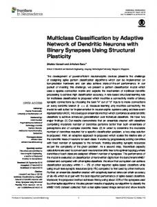
for brevity we show in the final column the number of classes that were removed before the one-class classifier became better than the two-class one. For all but two of the datasets shown in Table 3, there exists a point where it is better to use the one-class classifier over the two-class one. This is not unexpected: as the number of non-target classes is reduced, their coverage diminishes until it is no longer worthwhile to use them to define a boundary around the target class. For the two datasets where this is not the case, arrhythmia and primary-tumor, the density estimate does not appear to form a good model of the data for either classifier and the AUC is relatively low in both cases. Graphing the results for an individual dataset, such as shown for the audiology dataset in Figure 7, we find that the weighted AUC continually decays as we remove classes from the training data. Of course, the one-class classifier maintains a constant AUC because it does not use non-target data during training. The shape of decay shown in Figure 7 is typical of the datasets in Table 3. From the results in this section we can say that where there are limited non-target classes available at training time, thus increasing the potential for a novel class to appear that is dissimilar from any existing non-target class, oneclass classification should be used in preference to two-class classification. Note that in this situation it may also be beneficial to combine the classifiers in an ensemble—so available outlier training data can be utilised—but we have not investigated this option yet.
5
Conclusions
In this paper we have described how multi-class, two-class and one-class classifiers can be compared to each other by setting up identical test sets and employing the weighted AUC to compare their predictive performance in verification
11 0.95
Two-class classification One-class classification
Weighted AUC
0.9
0.85
0.8
0.75
0.7 0
5
10 Number of class labels removed
15
20
Fig. 7. Number of classes removed versus weighted AUC for the audiology dataset.
problems with novel classes. We have provided empirical data for each classification technique—Na¨ıve Bayes and the corresponding one-class model—using 27 UCI datasets. Using the results of our experiments, we are able to provide the following advice for use of each classifier in verification problems: – If no novel classes are expected after the classifier has been trained one should use multi-class classification without relabelling. – If novel classes are expected, then the training data should be relabelled to ‘target’ and ‘outlier’, where the former is the single class we are attempting to verify, and the latter contains all other classes relabelled to a single combined class. If there is a limited number of non-target classes, or they do not sufficiently cover possible novel cases for some other reason, then one should use one-class classification. Otherwise, one should use two-class classification. In situations where it is unclear whether to use one-class or two-class classification, it may be possible to combine the two classification methods in an ensemble. However, we have not performed any tests regarding this approach, and leave it as a possible avenue for future work. Future work could also include extending empirical results to other learning algorithms. Moreover, we feel it would be interesting to explore further the relationship between the number of non-target instances (rather than the number of classes) and the accuracy of the two-class classifier relative to the one-class classifier.
12
References 1. A. Asuncion and D. Newman. UCI machine learning repository, 2007. 2. M. Koppel and J. Schler. Authorship verification as a one-class classification problem. In Proceedings of the 21st International Conference on Machine Learning, pages 489–495, New York, NY, USA, 2004. ACM Press. 3. M. Nisenson, I. Yariv, R. El-Yaniv, and R. Meir. Towards behaviometric security systems: Learning to identify a typist. In Proceedings of the 7th International Conference on Principles and Practice of Knowledge Discovery in Databases, pages 363–374, Berlin, Germany, 2003. Springer-Verlag. 4. L. Tarassenko, P. Hayton, N. Cerneaz, and M. Brady. Novelty detection for the identification of masses in mammograms. In Proceedings of the Fourth International IEEE Conference on Artificial Neural Networks, pages 442–447, London, England, 1995. IEEE. 5. I. H. Witten and E. Frank. Data Mining: Practical machine learning tools and techniques. Morgan Kaufmann, San Francisco, USA, 2nd edition, 2005. 6. E. Yu and S. Cho. Novelty detection approach for keystroke dynamics identity verification. In Proceedings of the 4th International Conference on Intelligent Data Engineering and Automated Learning, pages 1016–1023, Berlin, Germany, 2003. Springer.