Improved Shortest Path Algorithms for Nearly Acyclic Graphs - CiteSeerX

Improved Shortest Path Algorithms for Nearly Acyclic Graphs

A thesis submitted in partial fulfilment of the requirements for the Degree of Doctor of Philosophy in Computer Science in the University of Canterbury by Shane Saunders

University of Canterbury 2004

This thesis is dedicated to my parents.

Abstract Dijkstra’s algorithm solves the single-source shortest path problem on any directed graph in O(m + n log n) worst-case time when a Fibonacci heap is used as the frontier set data structure. Here n is the number of vertices and m is the number of edges in the graph. If the graph is nearly acyclic, then other algorithms can achieve a time complexity lower than that of Dijkstra’s algorithm. Abuaiadh and Kingston gave a single source shortest path algorithm for nearly acyclic graphs with O(m + n log t) worst-case time complexity, where the new parameter t is the number of delete-min operations performed in priority queue manipulation. For nearly acyclic graphs, the value of t is expected to be small, allowing the algorithm to outperform Dijkstra’s algorithm. Takaoka, using a different definition for acyclicity, gave an algorithm with O(m + n log k) worstcase time complexity. In this algorithm, the new parameter k is the maximum cardinality of the strongly connected components in the graph. This thesis presents several new shortest path algorithms that define trigger vertices, from which efficient computation of shortest paths through underlying acyclic structures in the graph is possible. Various definitions for trigger vertices are considered. One definition decomposes a graph into a unique set of acyclic structures, where each single trigger vertex dominates a single corresponding acyclic structure. This acyclic decomposition can be computed in O(m) time, thus allowing the single source problem to be solved in O(m + r log r) worst-case time, where r is the resulting number of trigger vertices in the graph. For nearly acyclic graphs, the value of r is small and single-source can be solved in close to O(m) worst-case time. It is possible to define both monodirectional and bidirectional variants of this acyclic decomposition. This thesis also presents decompositions in which multiple trigger vertices dominate a single acyclic structure. The trigger vertices of such decompositions constitute feedback vertex sets. If trigger vertices are defined as a set of precomputed feedback vertices, then the all-pairs shortest path problem can be solved in O(mn + nr 2 ) worst-case time. This allows all-pairs to be solved in O(mn) worst-case time when a feedback vertex set smaller than the square root of the number of edges is known. For suitable graph types, these new algorithms offer an improvement on the time complexity of previous algorithms.

Table of Contents

List of Algorithms

ix

Chapter 1:

Introduction

1

Chapter 2:

Background Information

6

2.1

Basic Concepts . . . . . . . . . . . . . . . . . . . . . . . . . . .

6

2.2

Graph Terminology . . . . . . . . . . . . . . . . . . . . . . . . .

9

2.3

Graph Data Structures . . . . . . . . . . . . . . . . . . . . . . .

10

2.4

Dijkstra’s Algorithm . . . . . . . . . . . . . . . . . . . . . . . .

12

2.5

The Fibonacci Heap and Amortised Cost Analysis . . . . . . . .

17

2.6

A History of Different Shortest Path Algorithms . . . . . . . . .

19

Chapter 3:

Research Outline

27

3.1

The Research Area . . . . . . . . . . . . . . . . . . . . . . . . .

27

3.2

Related Work . . . . . . . . . . . . . . . . . . . . . . . . . . . .

30

3.3

An Overview of Existing Algorithms . . . . . . . . . . . . . . .

32

3.4

Possible Improvements to Existing Algorithms . . . . . . . . . .

35

Chapter 4:

Using Acyclic Decompositions to Compute Shortest Paths Efficiently

38

4.1

Computing Shortest Paths by Tree Decomposition . . . . . . . .

38

4.2

Computing Shortest Paths by Acyclic Decomposition . . . . . .

44

4.3

Computing Shortest Paths by Bidirectional Acyclic Decomposition 55

4.4

An Efficient Algorithm for Computing the Acyclic Decomposition of a Graph . . . . . . . . . . . . . . . . . . . . . . . . . . .

Chapter 5: 5.1

72

Using Feedback Vertex Sets to Compute Shortest Paths Efficiently 80

A New All-Pairs Shortest Path Algorithm Employing Feedback Vertices . . . . . . . . . . . . . . . . . . . . . . . . . . . . . . .

80

5.2 Applying Acyclic Decomposition Trigger Vertices as Feedback Vertices . . . . . . . . . . . . . . . . . . . . . . . . . . . . . . . 87 Chapter 6:

Multidominator Sets

92

6.1 Disjoint 2-dominator Sets . . . . . . . . . . . . . . . . . . . . . 92 6.2 Defining k-Dominator Set Covers . . . . . . . . . . . . . . . . . 105 6.3 A k-Dominator Set Cover Algorithm . . . . . . . . . . . . . . . 112 6.4 Restricted k-Dominator Set Cover Algorithms . . . . . . . . . . 126 6.5 Applying k-Dominator Set Cover Trigger Vertices as Feedback Vertices . . . . . . . . . . . . . . . . . . . . . . . . . . . . . . . 130 6.6 A Summary of the Different Types of Dominator Sets . . . . . . 133 Chapter 7: Experimental Results 135 7.1 Experimental Methodology and Setup . . . . . . . . . . . . . . . 135 7.1.1 7.1.2

Parameters Affecting Algorithm Performance . . . . . . 135 Generating Random Graphs . . . . . . . . . . . . . . . . 137

7.1.3 Algorithm Implementation Details . . . . . . . . . . . . . 140 7.2 Details of Experiments Performed . . . . . . . . . . . . . . . . . 141 7.3 Results and Analysis . . . . . . . . . . . . . . . . . . . . . . . . 145 7.3.1 7.3.2 7.3.3

Decomposition Effectiveness . . . . . . . . . . . . . . . . 145 Single-Source Results for Sparse Random Graphs . . . . 154 Single-Source Results for Graphs Favouring Acyclic De-

7.3.4

composition . . . . . . . . . . . . . . . . . . . . . . . . . 164 All-Pairs Results for Sparse Random Graphs . . . . . . . 167

7.3.5

A Summary of Experimental Results . . . . . . . . . . . 168

Chapter 8: Summary and Conclusions 171 8.1 Acyclicity Measures . . . . . . . . . . . . . . . . . . . . . . . . . 171 8.2 New Algorithms Contributed . . . . . . . . . . . . . . . . . . . . 176 8.3 Future Research . . . . . . . . . . . . . . . . . . . . . . . . . . . 179 References

182

Appendix A: Publications

186

viii

List of Algorithms 2.1 3.1

Dijkstra’s Algorithm . . . . . . . . . . . . . . . . . . . . . . . . GSS Algorithm . . . . . . . . . . . . . . . . . . . . . . . . . . .

14 34

4.1 4.2

First Stage of the Tree GSS Algorithm . . . . . . . . . . . . . . Second Stage of the Tree GSS Algorithm (Continues from Algo-

40

4.3 4.4

rithm 4.1) . . . . . . . . . . . . . . . . . . . . . . . . . . . . . . 42 Computing the 1-Dominator Set . . . . . . . . . . . . . . . . . . 49 Single-Source Algorithm Using Topologically Ordered Acyclic

4.5

Parts . . . . . . . . . . . . . . . . . . . . . . . . . . . . . . . . . 52 Computing the Bidirectional 1-Dominator Set . . . . . . . . . . 60

4.6 4.7

Bidirectional 1-Dominator GSS Algorithm . . . . . . . . . . . . 67 Computing 1-Dominator Decomposition in O(m) Worst-Case Time . . . . . . . . . . . . . . . . . . . . . . . . . . . . . . . . . 73

5.1 5.2

First Stage of the FVS All-Pairs Algorithm . . . . . . . . . . . . Second Stage of the FVS All-Pairs Algorithm . . . . . . . . . .

5.3 6.1 6.2

Bidirectional 1-Dominator Pseudo-Graph Computation . . . . . 89 Disjoint Single-Source Algorithm . . . . . . . . . . . . . . . . . 96 Computing a Disjoint 2-Dominator Set . . . . . . . . . . . . . . 100

6.3 6.4

Computing the Forward k-Dominator Set . . . . . . . . . . . . . 116 A function for Obtaining Bidirectional k-Dominator Acyclic Sets 122

6.5 6.6 6.7

Computing the Restricted k-Dominator Set . . . . . . . . . . . . 126 Computing a Restricted k 0 -Dominator Set . . . . . . . . . . . . 129 Computing the i-Dominator Set Optimal in |T (i)| . . . . . . . . 131

ix

83 85

Acknowledgments I would like to thank my supervisor, Tadao Takaoka, for the time he spent proof reading and the invaluable advice he gave which considerably improved the quality of this work. Many thanks also to all others in the Department of Computer Science and Software Engineering who have been of assistance over the years. I also acknowledge the anonymous reviewers of my published work for their constructive comments that helped contribute to the clarity of this thesis. Finally, I especially would like to thank my parents for all their support and encouragement.

x

Chapter 1

Introduction Shortest paths, or close to shortest paths, are commonly used in everyday situations. The use of shorter paths occurs naturally when travelling between two locations, whether this is travel from one room to another, from one street address to another, or from one city to another. Taking a long path typically makes no sense, since doing so results in time being wasted. Thus, shorter paths are preferred for reasons of efficiency. To achieve the greatest efficiency when travelling between two points, it is necessary to take a path that is shortest among all possible paths; that is, the shortest path. Generally speaking, a shortest path is one of minimal cost. The problem of computing shortest paths commonly arises when the most cost-efficient route through a transportation or communication network needs to be found. In the case of transportation, cost may be represented by a combination of factors, including distance travelled, time spent, fuel used, tolls paid, or many other factors. The exact definition being used for cost depends on the specific problem being solved. While shorter paths tend to be used naturally, determining truly shortest paths allows more efficient use of networks. Solving shortest paths by plain intuition is not always guaranteed to obtain the correct result. The truly shortest path, or that of minimum cost, is not always the most obvious choice. For example, consider finding the shortest path in order to minimise the time spent travelling between two locations in a city. Here cost is measured in terms of the time spent travelling. The shortest path may require taking a detour in order to avoid traffic congestion. Such a path can be completely different from the path that is shortest in terms of distance travelled. Even with cost defined as distance travelled, the correct choice of shortest path may be counter-intuitive. Furthermore, large shortest path problems are typically too complex to solve accurately by hand. By computing shortest paths, rather than using intuition, a correct result can always be obtained. Shortest path problems in general are described using the concept of a 1

B

10

D 5

4 A

3

1

6

2 4

C

F 2

E

Figure 1.1: An example of a directed graph consisting of six vertices (A, B, C, D, E, F) and nine edges. The edges in this graph are weighted; that is, each edge has an associated cost.

graph. A graph is a set of points and connections between these points; as seen in Figure 1.1. Each point in the graph is called vertex, and a connection between two points is called an edge. Graphs can be used to model many problems. Consider a transportation network consisting of several cities and the roads linking them. The corresponding graph for such a network represents each city as a vertex, and each road as an edge. Similarly, the vertices in a graph may be used to represent computers in a computer network, in which case the edges of the graph represent the communication links connecting computers. A graph may be either directed or undirected. The edges in an undirected graph have no direction associated with them, and can be thought of as allowing travel in both directions. In contrast, the edges in a directed graph have an associated direction, which can be thought of as specifying the direction of travel. The graph shown in Figure 1.1 is a directed graph. Think of edges in a directed graph as being one-way, and edges in an undirected graph as two-way. The edges of a graph can be weighted, in which case each edge has an associated cost. In the case of a transportation network, this cost may be the distance along a road between two vertices. Most shortest path problems are represented using directed graphs, since the cost from one vertex to another may be different in the opposite direction. The edges in a graph form paths connecting vertices. Any such path similarly has an associated cost (or distance), which corresponds to the sum of costs of edges along the path. The existence of alternative paths between a pair of vertices in a graph 2

provides the possibility of some paths being shorter than others in terms of their associated distance. Hence, the problem of determining which paths are the shortest arises. Shortest path problems can be solved by following an easily repeatable list of steps. Such a list of steps is called an algorithm. In general, an algorithm is a list of steps that are performed to accomplish a given task. Thus, a shortest path algorithm is a list of steps that describes how to compute a shortest path. Computers are able to perform the many steps described by an algorithm very quickly, and are therefore well suited to solving problems such as shortest paths. In order to solve a particular kind of problem, a computer must be provided with an algorithm describing how to compute the solution to the problem. It is possible to have different algorithms for solving the same kind of problem. One algorithm may use a more efficient approach to solve a problem, thereby solving the problem is less time compared to another algorithm. By devising algorithms that work more efficiently, the time required to solve problems can be decreased. In this sense, devising a more efficient shortest path algorithm will allow shortest paths to be computed in less time. This is important because the amount of time needed to compute shortest paths increases as shortest path problems become larger. A more efficient algorithm sees a much slower growth in its associated processing time compared to an inefficient algorithm. As a result, efficient algorithms tend to perform significantly faster than inefficient algorithms for increasingly larger problem sizes. Using a more efficient algorithm often achieves greater speedup than the alternative of purchasing a faster computer. Obtaining more efficient shortest path algorithms is especially important in cases where shortest paths need to be computed repeatedly, or need to be determined very quickly. For example, a computer’s knowledge of shortest paths through a communication network may need to be updated frequently as the conditions on the network keep changing. Similarly, emergency service vehicles may require the shortest path through a city to be computed very quickly as traffic conditions change. With increasingly larger problems arising, there is a need for more efficient algorithms. This requires that theoretical research is undertaken to enhance our understanding of shortest path problems and algorithm efficiency. 3

Some special kinds of shortest path problems can be solved more efficiently than standard shortest path problems. One such kind of problem arises when solving a shortest path problem on a directed graph that contains no cycles; that is, an acyclic directed graph. A cycle is a path through the graph that arrives back at the first vertex on the path. If there are no cycles, then shortest paths become easier to compute. As an example, consider a network of paths on a mountain slope and the requirement that only downhill travel is allowed, but never uphill or level travel. The directed graph representing such paths is acyclic, since it is impossible to get back to a previously visited point when travelling on strictly downhill paths. Since every path proceeds downhill, computing the shortest path is easier than in cases where both uphill and downhill travel is allowed. Conventional shortest path algorithms do not take this strictly downhill travel into account when computing shortest paths, and perform as they would on any graph. In contrast, specialised shortest path algorithms that are designed to take into account strictly downhill travel will perform faster on such graphs. It happens that there is such an algorithm for acyclic graphs. There are also specialised shortest path algorithms for other kinds of graphs. In order to solve a particular kind of shortest path problem more efficiently, an appropriate algorithm must first be invented. The motivation of this thesis is to design specialised shortest path algorithms for use on nearly acyclic graphs. A nearly acyclic graph is a graph that contains relatively few cycles for its size. One kind of nearly acyclic graph can be visualised by extending the strictly downhill example, described earlier, to allow some uphill paths. In this nearly downhill analogy, most, but not all, paths in the graph are downhill. Since such graphs are not strictly downhill, an efficient strictly downhill shortest path algorithm cannot be used. Therefore a standard shortest path algorithm would normally be used to solve shortest paths in such graphs. However, given that most of the graph is downhill, there should be some more efficient way to solve shortest paths. This requires a new specialised algorithm for nearly downhill graphs to be invented; that is, an algorithm for nearly acyclic graphs. By designing new shortest path algorithms for nearly acyclic graphs these kinds of problems may be solved almost as efficiently as problems on acyclic graphs. This thesis presents several new algorithms for solving shortest paths on 4

nearly acyclic graphs. This kind of theoretical research extends on the existing knowledge about how shortest paths can be solved efficiently, and can lead to even better shortest path algorithms being developed. The new algorithms contributed by this thesis are theoretically faster than conventional shortest path algorithms when a graph is nearly acyclic. There is much potential for such specialised algorithms to be of practical benefit if any real-world shortest path problems on nearly acyclic graphs are discovered in the future.

5

Chapter 2

Background Information Shortest path algorithms have a long history, with the computation of shortest paths being one of the most well studied graph optimisation problems. Many shortest path algorithms exist for solving various forms of shortest path problems. Before discussing some of these different algorithms, some basic concepts related to shortest paths are described in Section 2.1. Likewise, important graph terms used throughout this thesis are defined in Section 2.2. Section 2.3 describes the data structures used by shortest path algorithms to represent graphs. Section 2.4 then reviews the classical textbook algorithm of Dijkstra [8], which provides the foundation of many shortest path algorithms. A description of the Fibonacci heap used in efficient implementations of Dijkstra’s algorithm is provided in Section 2.5, along with some details on the concept of amortised analysis. Following this, Section 2.6 describes other important historical achievements related to the computation of shortest paths. 2.1

Basic Concepts

Formally, a shortest path problem is represented as a graph G = (V, E), consisting of a set of vertices V and a set of edges E. Various algorithms exist for solving shortest paths, depending on the type of graph involved. Firstly, a graph may be either directed or undirected, corresponding to whether the edges e ∈ E have a direction associated with them. Secondly, a graph may

be either weighted or unweighted. In a weighted graph, each edge e ∈ E has an associated weight, or cost, c(e). A weighted graph may use arbitrary realvalued edge costs, or be limited to integer edge costs. Furthermore, a weighted graph may allow both positive and negative edge costs, or be restricted to only non-negative edge costs. Graphs can be further categorised according to the structure formed by their edges. This leads to families of graphs, such as planar graphs, acyclic graphs, strongly connected graphs and bipartite graphs. 6

Provided with a graph, one may need to find the shortest paths from a single starting vertex s to all other vertices in the graph. This is known as the single-source shortest path problem. Viewed as a whole, the shortest paths from s to other vertices form a shortest path tree covering every vertex in the graph. A larger problem is to find shortest paths between all pairs of vertices in the graph. This is known as the all-pairs shortest path problem. Algorithms exist for solving both the single-source problem and the all-pairs problem. One way to solve all-pairs is by solving single-source from all possible source vertices in the graph. Dijkstra’s algorithm [8], invented in 1959, provides an efficient approach to solving single-source on positively weighted directed graphs with real-valued edge costs. Many of today’s shortest path algorithms are based on Dijkstra’s approach. There is also the simple problem of single-pair shortest paths, where the shortest path between a single source-vertex and a single destination-vertex must be determined. However, in the worst case, this kind of problem is as difficult to solve as single-source. In order to make an accurate comparison of various shortest path algorithms, the model of computation under which they work needs to be taken into account. Computational models provide a machine independent method of analysing and comparing algorithm efficiency. Some efficient algorithms are achieved by allowing a more powerful computational model. Shortest path algorithms are generally analysed using two variants of the Random Access Machine (RAM) model [4]. The first variant, called the comparison-addition model, works with real-valued edges costs and assumes that comparison and addition are the only operations allowed on edge weights and numbers derived from them. Each operation is assumed to take constant time. The second variation, called the word RAM model, works with integers (machine words) of a limited number of bits. On top of addition and comparison, this model provides other operations such as subtraction, bit shifts, and logical bit operations. However, this also assumes that a single machine word contains enough bits to represent any vertex number. Once again, each operation is assumed to take a constant amount of time. Sometimes constant-time multiplication is also assumed. Most shortest path algorithms work under the standard comparisonsaddition model, but some faster algorithms have been achieved using the more 7

powerful word RAM model. Other algorithms achieve improved efficiency by using subtraction on top of the standard comparison-addition model operations, and sometimes even multiplication and division. All of the algorithms developed in this thesis assume the standard comparison-addition model. In any computational model, the time taken by an algorithm is proportional to the number of constant-time operations performed, and can be described as function of certain parameters such as the size of the problem. With constant factors ignored, this function is called the time complexity of the algorithm. The time complexity of an algorithm represents the functional order of its running time, and describes how the running time grows in proportion to certain parameters such as problem size. Time complexity is expressed using the big-O notation. If an algorithm runs in O(f (n)) time, where n is the problem size, then its actual running time g(n) cannot exceed the functional order of f (n); that is, there is some constant c such that cf (n) > g(n) for all n. Time complexity provides a useful metric for comparing algorithms. Consider two algorithms A1 and A2 with time complexities of O(n) and O(n2 ) respectively. Suppose that the actual running times are described by the functions g1 (n) = 1000n and g2 (n) = n2 respectively. Here A1 has a much larger constant factor associated with its running time. However, because of the lower time complexity, the time taken by A1 grows more slowly than the time taken by A2 as n increases. While A2 may be faster for small values of n, the fact that A1 is theoretically more efficient means that A1 is faster than A2 for increasingly large values of n; in this case n > 1000. The worst amount of time that an algorithm will spend on arbitrary input is described by its worst-case time complexity. This is the typical time complexity measure that is obtained when analysing algorithms. Another measure is the average-case (or expected ) time complexity, which relates to the average (or expected) running time of an algorithm on arbitrary input. Sometimes the best-case time complexity may be considered. The research presented in this thesis is primarily concerned with the worst-case time complexity analysis of algorithms. Average-case analysis can prove useful when comparing the practical performance of algorithms, but does not take into account the worst amount of time that an algorithm may spend. For this reason, worst-case analysis is preferred for the theoretical comparison of algorithms. 8

In summary there are many factors associated with shortest path algorithms. First, there is the type of graph on which an algorithm works — directed or undirected, real-valued or integer edge costs, and possibly-negative or non-negative edge-costs. Furthermore, there is the family of graphs on which an algorithm works — acyclic, planar, and strongly connected, to name some. Then there is the kind of shortest path problem being solved — single-source or all-pairs. Finally, there is the computational model under which algorithms work to achieve their result, and whether this result is associated with the worst-case or average-case time complexity. All of the shortest path algorithms presented in this thesis assume directed graphs with non-negative real-valued edge costs. Furthermore, the standard comparison-addition model is used. The aim is to develop algorithms that offer an improved worst-case time complexity when applied on a family of graphs called nearly acyclic graphs. The textbook by Aho, Hopcroft, and Ullman [4] provides further introduction to shortest path algorithms and algorithm analysis. Another good algorithms text by Cormen, Leiserson, and Rivest [6] contains descriptions of many algorithms. Details such as graph theory terms related the algorithms mentioned in this thesis can be found in Gibbons [14]. 2.2

Graph Terminology

This section reviews some basic graph theory terms that are important to understanding some of the shortest path algorithms described later. One of the most basic graph theoretic definitions related to shortest paths is that of a path. Firstly, the notation u → v denotes the existence of a directed edge from vertex u to vertex v. Under this notation, v0 → v1 → . . . → vl represents a directed path of length l, where each vi for 0 ≤ i ≤ l is a vertex on the path. Here v0 is the first vertex on the path, and vl is the last vertex

on the path. A path can alternatively be denoted as an ordering of vertices (v0 , v1 , v2 , . . . , vl ) such that there exists an edge vi → vi+1 for all 0 ≤ i ≤ l − 1. A path whose first and last vertices are the same is called a cycle; that is, a path of the form (v, w1 , w2 , . . . , wl , v), where l ≥ 0.

One of the simplest graph properties is that of acyclicity. The concept

of acyclicity is used throughout this thesis. A graph is acyclic if it does not contain any cycles. The vertices of a directed acyclic graph can be topologically 9

ordered. A topological ordering (v1 , v2 , . . . vk ) of k vertices satisfies the property i < j wherever there exists an edge vi → vj for any 1 ≤ i ≤ k and 1 ≤ j ≤ k. As will be seen, a topological ordering of vertices can be used to compute shortest paths more easily. It is possible to compute a topological ordering of the vertices in a directed acyclic graph in linear time. One method is to take the reverse of the postorder of vertices produced by a depth first-search of a nearly acyclic graph. Another kind of graph property is that of planarity. A graph is planar if it can be drawn in a plane without any edges crossing. It has been proved that any planar undirected graph satisfies the inequality m ≤ 3n − 6 for n ≥ 3. Consequently, planar directed graphs satisfy m < 6n − 12. Therefore, the number of edges m in a planar graph is O(n). The property of planarity is analogous to that of acyclicity in that shortest paths become easier to compute. A further structural property of graphs is connectivity. A graph is strongly connected if there exists a path from u to v for all pairs of vertices u and v in the graph. A graph that is not strongly connected can be partitioned into a set of maximal strongly connected subgraphs, called strongly connected components (or SC components for short). As will be seen, the property of strong connectivity has also been used to speed up shortest path computations. 2.3

Graph Data Structures

Graph algorithms need to have efficient access to the vertices and edges of a graph stored in the computer’s memory. There are two common data structures used for storing a graph in computer memory. This section provides an overview of these. For simplicity, it will be assumed that the graph is directed, and the vertices of the graph are numbered from 1 to n. The first kind of data structure used is the adjacency matrix. This is simply an n by n matrix A stored as a two-dimensional array. Entry A[v, w] in the matrix holds the distance of the edge v → w. If the edge v → w does not exist, then A[v, w] is set to infinity; which may be represented using some special value such as a negative value. Alternatively, a separate Boolean adjacency matrix C can be used, with C[v, w] = 1 if an edge exists from v to w, and C[v, w] = 0 otherwise. An adjacency matrix data structure requires O(n2 ) space. This is acceptable for storing dense graphs, which contain around O(n2 ) 10

edges. However, for sparser graphs, which contain significantly fewer edges, the adjacency matrix is inefficient. The second kind of data structure used is the adjacency list. This represents the edges of the directed graph by using edge lists, and is more efficient for sparse graphs. In the adjacency list data structure, each vertex has an associated list which contains all of its outgoing edges. To represent an edge, each list item provides a target vertex number and the distance to that vertex. Thus, if edge v → w exists, then vertex v’s edge list contains an item whose

target vertex is w. The overall data structure takes the form of an array of n edge lists; and, with one list item per edge, requires just O(n + m) space. Each edge-list is normally implemented as a liked list. The liked-list may be singly- or doubly-liked depending on whether the data structure needs to support efficient the deletion of edges from the graph. In addition, it is possible to maintain a list of incoming edges to facilitate reverse traversal of edges. Both of these graph data structures have their advantages and disadvantages. The adjacency matrix requires O(n) time to traverse all the outgoing edges of a vertex v, since all n entries in row v of the matrix must be examined to see which edges exist. This is inefficient for sparse graphs since the number of outgoing edges j may be much less than n. In contrast, the adjacency list data structure allows all j outgoing edges to be traversed in just O(j) time simply by examining each edge in the list. Although the adjacency matrix is inefficient for sparse graphs, it does have an advantage when checking for the existence of an edge v → w, since this can be done in O(1) time by looking up array entry C[v, w]. In contrast, the same operation using an adjacency list data structure requires O(j) time since each of the j edges in vertex v’s list must be examined to see if the target is vertex w. The adjacency matrix can also be very favourable if the graph is frequently manipulated by repeatedly adding and deleting edges. This is because an edge can be added or deleted simply by writing to the appropriate entry in the matrix. However, the O(n2 ) space requirement for adjacency matrices severely limits its application to small or dense graphs. Given that most algorithms do not need to manipulate the graph or perform edge existence queries, the adjacency list data structure is suitable for most applications; especially if the graph is sparse. If the graph is dense, then the connection matrix data structure provides a reasonably ef11

ficient alternative. Many algorithms for dense graphs are in fact designed to work only with the connection matrix data structure. All of the shortest path algorithms developed in this thesis are intended for sparse graphs, and therefore assume that the graph is represented using the adjacency list data structure. Since outgoing edges are always accessed consecutively, each access to an outgoing edge takes O(1) time by traversing a vertices adjacency list. Using an array of n edge lists, the edge-list of a particular vertex is easily accessed O(1) time by looking up the corresponding array entry. 2.4

Dijkstra’s Algorithm

The following explanation of Dijkstra’s algorithm serves as a good starting point for describing how shortest paths are computed. Dijkstra’s algorithm computes the shortest paths from a starting vertex s to all other vertices in a non-negatively weighted directed graph G = (V, E), where V is the set of vertices in the graph, and E is the set of edges. Here V is given by the set integers {1, 2, . . . , n}. In the following description of Dijkstra’s algorithm,

OUT (v) is defined as the set of all vertices w such that there is a directed edge from vertex v to vertex w. The cost function c(v, w) ≥ 0 gives edge

cost from vertex v to vertex w. In general, where real-valued edge costs are assumed, Dijkstra’s algorithm works under the comparison-addition model of computation.

In solving a single-source shortest path problem, Dijkstra’s algorithm maintains a distance value d[v] for each vertex v in the graph. During the computation, the value of d[v] is equal to the distance of the shortest known path from s to v. Dijkstra’s algorithm determines increasingly shorter paths to each vertex v, and eventually reduces each distance value d[v] to a final value corresponding to the actual shortest path distance from s to v. Dijkstra’s algorithm distinguishes between vertices by placing explored vertices either in a solution set S or a frontier set F . Only unexplored vertices remain outside S and F . An example snapshot of Dijkstra’s algorithm is provided in Figure 2.1. The solution set S holds vertices v for which the shortest path distance is known; with d[v] being equal to the final shortest path distance. In contrast, the frontier set F holds vertices v for which the shortest 12

S

3 5

0

8

5

S

F

5

1 2

2

14

3

4

6

3

0

8

3

= minimum vertex

2

1

2

2

3

9

8

5

10 4

6

4

F

12

8 16

8

3

9

= untraversed edge = traversed edge = shortest path

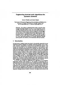
Figure 2.1: An example of the progress of Dijkstra’s algorithm. Solid edges and vertices indicate the traversed parts of the graph. Bold edges indicate shortest paths through S to vertices in F . Visited vertices v each have an associated shortest path distance label d[v] shown as a rectangular box. As illustrated, the minimum vertex in F (with distance label 8) moves from F to S and propagates shortest path distances onto adjacent vertices.

path distance is yet to be finalised, with d[v] being some tentative shortest path distance. Initially, Dijkstra’s algorithm only knows the shortest path distance to the starting vertex s, with d[s] assigned a shortest path distance of zero. Since the value of d[s] = 0 is final, vertex s is placed in the solution set. The edges leading from s provide paths to other vertices v ∈ OUT (s). Dijkstra’s

algorithm places these vertices v ∈ OUT (s) in the frontier set F , setting the distance value d[v] equal to c(s, v). During the computation, the distance value d[v] for each vertex v ∈ F is

equal to the distance of the shortest path from s to v via vertices in S. Now, consider the vertex u ∈ F such that d[u] is minimum; simply referred to as

the minimum vertex. As for any vertex, the value of d[u] is the distance of the shortest path to u via vertices in S. In addition, no shorter path to u exists, since this would require the use of some other vertex in v ∈ F with d[v] < d[u]. Therefore the value of d[u] for the minimum vertex u is final. Thus, to proceed, Dijkstra’s algorithm deletes the minimum vertex u from F

and places it in S. With u being moved to S, the tentative shortest path distance d[v] of vertices v ∈ OUT (u) must be updated. Only those vertices 13

Dijkstra’s Algorithm

Algorithm 2.1. 1. 2. 3.

S = {s}; F = ∅; for each v in OUT (s) do {

4. 5.

add v to F with d[v] = c(s, v); }

6. 7. 8.

while F is not empty do { select u such that d[u] is minimum among u in F ; remove u from F ; /* delete min */

9. 10.

add u to S; for each v in OUT (u) and not in S do {

11. 12. 13.

if v is not in F then { d[v] = d[u] + c(u, v); add v to F ; /* insert */

14. 15.

} else {

16. 17. 18. 19.

d[v] = min(d[v], d[u] + c(u, v)); /* decrease key */ } } }

v ∈ OUT (u) such that v ∈ / S are considered since d[v] is already final for vertices v ∈ S. If v ∈ F , then the shortest path distance is updated by the

operation d[v] ← min(d[v], d[u]+c(u, v)). Thus, where the edge u → v provides a shorter path, the value of d[v] will be updated to reflect this. Whereas, if v∈ / F , then vertex v is inserted into F with an initially assigned shortest path distance of d[v] = d[u] + c(u, v). Dijkstra’s algorithm repeatedly performs this process of moving the minimum vertex from F to S and updating shortest path distances of neighbouring vertices. Eventually, all reachable vertices v will be explored and moved to S, with d[v] corresponding to the distance of the shortest path to v. Hence, a solution to the single-source shortest path problem is obtained. 14

Dijkstra’s algorithm can additionally construct the shortest path tree associated with the computed shortest path distances. This is done by maintaining a value p[v] for each vertex v, and setting p[v] equal to the preceding (or predecessor) vertex on the shortest path to v. Each time the minimum vertex u updates the shortest path to some vertex v, the value of p[v] is assigned u. When Dijkstra’s algorithm terminates, p[v] specifies the parent of vertex v in the shortest path spanning tree. A critical part of Dijkstra’s algorithm is the selection of the minimum vertex from F . This requires that the vertices in F be organised in some kind of a data structure. The way in which this data structure keeps track of the minimum vertex determines the computational efficiency of Dijkstra’s algorithm. There are three primary operations that this data structure must support: • delete min(): For locating and removing the minimum vertex from F . • insert(v, k): For inserting a vertex v into F with a key k equal to the assigned tentative distance value d[v]. • decrease key(v, k): For decreasing the distance d[v] of a vertex v in F , where they key k equals the new value for d[v].

Dijkstra’s algorithm eventually visits every vertex in the graph that is reachable from S. Assuming that all vertices are reachable, Dijkstra’s algorithm performs a total of n insert and n delete min operations. The number of decrease key operations is O(m) since this corresponds to the number of edges in the graph. The data structure used determines the resulting time-complexity of Dijkstra’s algorithm. A simple, but rather inefficient, data structure can be implemented using a one-dimensional array whose entries contain the key value of each vertex in F . With no sorting of key values, this can be implemented to support the insert and decrease key operations in O(1) worst-case time. The inefficiency arises when performing a delete min operation. Locating the minimum vertex requires up to n array entries being scanned, spending at worst O(n) time per delete min. This results in an O(n2 ) worst-case time complexity for Dijkstra’s algorithm; with n×O(1) insert , n×O(n) delete min and m×O(1) decrease key operations. Note that m is, at worst, equal to n(n − 1). This is efficient for 15

dense graphs, where the number of edges m that must be scanned is O(n2 ), but is inefficient for sparser graphs. For sparse graphs, a more efficient data structure is the binary heap [37]. This can also be implemented using 1-dimensional arrays, and, with at most n items in the heap, supports each of the operations insert, delete min and decrease key in O(log n) worst-case time. The result is that Dijkstra’s algorithm runs in O(m log n) worst-case time. This time complexity provides better efficiency for sparse graphs, where m is closer to O(n). However, for 2

n dense graphs, where m is greater than O( log ), the O(n2 ) version of Dijkstra’s n algorithm is actually more efficient.

The inefficiency of the binary heap form of Dijkstra’s algorithm was overcome with the invention of a new data structure called the Fibonacci heap [12]. The Fibonacci heap supports the insert and decrease key operations in O(1) time, and the delete min operation in O(log n) time. The cost of these operations is based on amortised analysis, which guarantees that this is the observed cost over a sequence of operations that returns the heap back to its initial empty state. A detailed description of Fibonacci heaps and amortised analysis is given in Section 2.5. When using a Fibonacci heap, a run of Dijkstra’s algorithm involves n O(1) insert operations, n O(log n) delete-min operations and m O(1) decrease-key operations. In summary, the Fibonacci heap gives Dijkstra’s algorithm a worst-case time complexity of O(m + n log n). Interestingly, this is the optimal time complexity for using Dijkstra’s algorithm to compute shortest paths on an arbitrary directed graph of n vertices and m edges containing positive real edge costs. This fact follows by noting that any implementation of Dijkstra’s algorithm requires at least O(m) time to scan all m edges, plus the O(n log n) lower time-bound [4] relating to sorting n real numbers, given that Dijkstra’s algorithm produces distances in sorted order. Although the Fibonacci heap provides the best worst-case performance for Dijkstra’s algorithm, binary heap implementations of Dijkstra’s algorithm perform better than Fibonacci heap implementations in practice. This is because the expected number of decrease-key operations is much less than O(m); refer to Noshita et al. [21]. Since the invention of the Fibonacci heap, other data structures supporting the optimal O(m + n log n) running time of Dijkstra’s algorithm have been invented. These include the relaxed heap [9], 2-3 heap 16

[28], and trinomial heap [29]. The O(m + n log n) time complexity obtained by the Fibonacci heap and equivalent data structures is optimal when using Dijkstra’s algorithm to solve shortest paths on positively weighted graphs in general. This result currently remains unimproved by any comparison-addition based single-source algorithm. It is an open problem as to whether the singlesource problem is as hard as sorting; that is, whether a comparison-addition based shortest-path algorithm is possible that beats the O(n log n) lower bound of sorting. 2.5

The Fibonacci Heap and Amortised Cost Analysis

The amortised cost of Fibonacci heap operations provides Dijkstra’s algorithm with a worst-case time complexity of O(m + n log n). This section provides a short description of the Fibonacci heap, and an overview of the concept of amortised analysis. A Fibonacci heap consists of a collection of trees. Unlike a binary heap, a Fibonacci heap allows each node in the tree to have more than just two children. The rank of a node is defined as the number of children that a node has, and the rank of a tree is defined as the number of children of the root node of the tree. The Fibonacci heap maintains at most one tree of each rank. A rank zero tree consists of a single node. A rank i tree is formed by combining two rank i − 1 trees. When inserting an item into a Fibonacci heap, a new node of rank zero is created to represent the item. This node can be regarded as a new rank zero tree in the Fibonacci heap. If a rank zero tree already exists, then, to maintain at most one tree of rank zero, the new and existing rank zero tree are merged together by making the root node with the smaller key a child of the other root node. This forms a tree of rank two, which may then need to be merged with an existing tree of rank two. In general a rank i tree is merged with any existing rank i tree to form a rank i + 1 tree, which may itself be merged, and so forth. It can be shown that this merging process results in no more than O(log n) trees. By this insertion process, the nodes of all trees are heap ordered, with the key of any node being smaller than that of its children. The overall amortised cost for any insert operation can be shown to be O(1). When a decrease-key operation occurs on a node, its key value may become smaller than that of its parent. To maintain heap order, the node and the 17

subtree rooted at it is trimmed from its parent, and merged back into the root level of the heap. This means that the parent node will have one less child than it is supposed to. The Fibonacci heap allows any node to lose at most one of its children. A node that has lost a child is marked to indicate this. If a marked node loses a child, then that node must also be trimmed from its parent. This process may propagate all the way up to the root node, and is called a cascading cut. A cascading cut results in a collection of trees of increasing rank to be merged back into the heap. The amortised cost of any decrease-key operation can be shown to be O(1). With heap-ordered trees, the minimum node resides at the root of one of the Fibonacci heap’s trees. During the insert and decrease-key operations, a pointer to the minimum root node in the heap is always maintained. When a delete-min operation occurs the minimum node is easily located using this pointer. With the minimum node located, it is trimmed from all its children (if any) and removed from the heap. The resulting collection of child trees must then be merged back into the heap, and the minimum node pointer updated. Overall, delete-min can be shown to have an amortised cost of O(log n). Amortised cost analysis [33] works on the principle that each heap operation invests or removes some potential from the heap. This potential takes the form of items ordered into the heap’s structure, and can be thought of as an investment; that is, the cost of ordering items into a heap structure provides an investment in being able to efficiently access items later on. The amortised cost of a heap operation is defined as amount of time spent minus the amount of potential invested. Any sequence of heap operations that returns the heap back to its initially empty state will result in no overall change in the heap’s potential since the potential of an empty heap is fixed. Therefore, the total of the amortised costs of such heap operations is the same as the total of their actual costs. To see the correctness of this kind of amortised analysis in more detail, let Φi denote the potential of the heap after heap operation i. Similarly, let si denote the amortised cost of the ith heap operation, and ai the actual cost. Here the actual cost of a heap operation can be thought of as the number of comparison operations performed on the key values of nodes in the heap. Thus, the amortised cost of a heap operation is the number of key comparisons 18

performed minus the change in potential. Expressed mathematically, si = ai − (Φi − Φi−1 ). The sum of the amortised costs of heap operations gives the overall amortised cost s:

s=

X

si

i

Similarly, summing actual costs of heap operations gives an overall actual cost a: X a= ai i

Considering the sum of amortised costs over N heap operations gives: s = s 1 + s2 + . . . + s N = (a1 − (Φ1 − Φ0 )) + (a2 − (Φ2 − Φ1 )) + . . . + (aN − (ΦN − ΦN −1 )) = a1 + a2 + . . . + an + (ΦN − Φ0 ) + ((Φ1 − Φ1 ) + (Φ2 − Φ2 ) + . . . (ΦN −1 − ΦN −1 )) = a1 + a2 + . . . + an + (ΦN − Φ0 ) = a + (ΦN − Φ0 ) Here the potential terms in the sum cancel, leaving ΦN − Φ0 , where Φ0 is the heap’s initial potential and ΦN is its final potential. If the sequence of heap operations returns the heap to its initial state, then the potential at the start and end is the same, giving Φn − Φ0 = 0. It thus follows that s = a; that is, the total amortised cost of heap operations is equal to the total actual cost. This is indeed the case for Dijkstra’s algorithm, since it starts and ends with an empty heap. Hence, based on the amortised cost of Fibonacci heap operations, Dijkstra’s algorithm proves to have a worst-case running time of O(m+n log n). All of the new algorithms developed in this thesis return to the same initially empty heap state, thus allowing the overall worst-case time to be determined from the amortised cost analysis of heap operations. Each uses a Fibonacci Heap, or equivalent data structure, to achieve their stated time complexity. 2.6

A History of Different Shortest Path Algorithms

The invention of Dijkstra’s algorithm provided an elegant method for computing single-source shortest paths efficiently. Many shortest paths algorithms based on Dijkstra’s approach have been seen since, as well as shortest path algo19

rithms based on other approaches. This section discusses the history of shortest path algorithms, focusing on algorithms for positively weighted directed graphs; in particular, algorithms that work under the comparison-addition model of computation. A broader survey of shortest path algorithms can be found in [38]. The different shortest path algorithms are most generally categorised according to the type of graph that they work on. While most shortest path algorithms work on directed graphs, there are some specifically designed for undirected graphs. Furthermore, the type of graphs that an algorithm works with may be restricted to certain assumptions, such as no negative edge costs, or no negative cycles within the graph. Among algorithms for a certain graph types, there are algorithms designed for dense graphs and algorithms designed for sparse graphs. An algorithm for dense graphs relates its performance to the number of vertices n in the graph. Thus, the time complexity of such algorithms is expressed as a function of the parameter n. In contrast, an algorithm for sparse graphs relates its performance to the number of edges m in the graph as well as the number of vertices. Here the time complexity is expressed as a function of both the parameters n and m. In addition to algorithms for dense and sparse graphs, there are specific families of graphs that an algorithm may work with: acyclic, planar, limited integer edge costs, and nearly acyclic, to name a few. Therefore, the time complexity of a shortest path algorithm may contain additional parameters which relate to particular graph properties. Such parameters may be a direct measure of some graph property, or a measure of the algorithm’s performance on a given graph. As described earlier, there are two main kinds of shortest path problems that are solved — single-source or all-pairs. Any single-source algorithm can be used to solve all-pairs by considering all possible source vertices. In addition, there are all-pairs only algorithms, which specifically solve all-pairs, but not single-source. There is also a third class of algorithms for computing single-pair shortest paths. Such single-pair algorithms are almost identical to single-source algorithms, but achieve a faster expected running time by ending shortest path computations once the shortest path to the destination vertex is known. The performance offered by an algorithm is categorised according to whether it is deigned for improved worst-case, average-case, or even best-case perfor20

mance. An algorithm that offers a very good average-case time complexity may in-fact have a very poor worst-case time complexity. There is also the computational model under which the algorithm’s time complexity is achieved. Usually, the comparison-addition model is assumed. However, some algorithms achieve their time complexity by assuming more powerful computational models such as the word-RAM model. An algorithm’s time complexity may also be derived from the amortised cost of data structure operations. Amortised cost analysis achieves a worst-case time complexity as the sum of the time taken by individual data structure operations whose time may vary during the running of the algorithm. Although the time of individual operations varies, their net effect results in a worst-case time expressed by amortised analysis. Amortised analysis needs to be taken into account if the internal performance of the algorithm is an issue. For example, amortised cost operations would be unsuitable in situations where an algorithm must make smooth progress toward computing a solution, in contrast to computing some parts quickly and some parts slowly. The classic shortest path algorithms, which were invented early on, are still in use today. Dijkstra’s algorithm [8], invented in 1959, for computing single-source shortest paths provides the foundation for many of today’s shortest path algorithms. Applying Dijkstra’s algorithm from every source vertex in the graph solves all-pairs. Floyd’s algorithm [10], invented in 1962, provides an alternative to Dijkstra’s algorithm when solving all-pairs on dense graphs. Remarkably, Dijkstra’s algorithm implemented with a Fibonacci heap, or equivalent data structure, remains the theoretically most efficient algorithm known for solving single-source on a non-negatively weighted directed graph. Dijkstra’s algorithm only works for graphs with non-negative edge weights. The classic Bellman-Ford algorithm (described in [6]) solves the more general problem, where edge weights may be negative, in O(mn) time. Algorithms that work on negative edge-weights are a separate topic. This thesis is mostly concerned with shortest path algorithms for non-negatively weighted directed graphs, particularly those derived from Dijkstra’s approach. Since the invention of Dijkstra’s algorithm, many shortest path algorithms have been seen. An early algorithm presented by Dantzig [7] achieved the same O(n2 ) worst-case time complexity of as the original version of Dijkstra’s algo21

rithm. Dantzig’s algorithm took a different approach by first sorting the edge lists of the graph. Like Dijkstra’s algorithm, Dantzig’s algorithm can solve single-source in O(m log n) time if implemented with a binary heap. However, because of the time required to sort the edges of the graph, Dantzig’s algorithm cannot achieve a worst-case time complexity better than O(m log n). Other early algorithms aimed to improve on the O(n2 ) and O(m log n) time complexities of Dijkstra’s algorithm. The d-heap data structure attributed to Johnson [18] (and also described in [32]) gave Dijkstra’s algorithm a time com). Since this time complexity is plexity of O(m logd n), where d = max(2, m n no worse than O(n2 ) on dense graphs where m is O(n2 ), the d-heap variant of Dijkstra’s algorithm improves on the O(m + n log n) time complexity of the binary heap variant. The achieved time complexity is alternatively expressed as O(min(m + n1+1/k , m log n)) where k is a fixed integer satisfying k ≥ 1. More recently, algorithms have aimed to improve on the O(m + n log n) time complexity obtained by the Fibonacci heap version of Dijkstra’s algorithm. Many algorithms exist for solving the all-pairs problem. Using the simple O(n2 ) variant of Dijkstra’s algorithm, the all-pairs shortest path problem can be solved in O(n3 ) worst-case time. A simpler algorithm provided by Floyd matched this O(n3 ) worst-case running time. In addition, Floyd’s algorithm works on graphs with negative edge-weights provided that there are no negative cycles. Negative cycles complicate the problem of solving shortest paths since a negative cycle may be taken infinitely many times producing a forever shorter path. The O(n3 ) worst-case time complexity of these approaches is acceptable when solving all-pairs on dense graphs. For sparse graphs, the O(m + n log n) variant of Dijkstra’s algorithm is a better choice, allowing all-pairs to be solved in O(mn + n2 log n) worst-case time. Here, the algorithm’s performance can be expressed in terms of the number of edges and vertices. This approach is always within the time complexity of Floyd’s algorithm since m is at worst O(n2 ). A path preserving graph reduction by Johnson [18], allows the O(mn + n2 log n) worst-case time complexity provided by Dijkstra’s algorithm to also be realised when solving all-pairs on negatively weighted directed graphs, assuming there are no negative cycles. Continued research asked whether the O(mn + n2 log n) time complexity achieved by Dijkstra’s algorithm for solving all-pairs could be improved upon. 22

This was partly answered when Hagerup [16] gave a worst-case time complexity of O(mn + n2 log log n) under the word-RAM type model for graphs with integer edge costs. Hagerup’s algorithm, extended on a word-RAM approach used by Thorup [34] to solve single-source in O(m) worst-case time on undirected graphs. Recently, Pettie [22] extended Hagerup’s result, to achieve O(mn + n2 log log n) worst-case time under the comparison-addition model for graphs with real edge costs. This currently stands as the best worst-case time complexity for solving all-pairs on directed graphs where edge weights are nonnegative real numbers, and m and n are the only parameters. Introducing other parameters allows some further improvement to the allpairs time complexity. Karger et al. [19] achieved an O(m∗ n + n2 log n) algorithm where m∗ is the number of edges participating in shortest paths, and is expected to be O(n log n) for most graphs. This provides a potential improvement for dense graphs, where many edges do not contribute to shortest paths. However, in effect, this only represents an average-case time complexity, since good values of m∗ refer to average graphs. The time complexity reverts to the worst case of O(mn + n2 log n) when m∗ is O(m). Algorithms that give good average-case performance appeared prior to this result. Using a similar approach to Dantzig’s algorithm [7], Spira [25] produced an all-pairs algorithm with an average-case running time of O(n2 log2 n). Later, Moffat and Takaoka [20] combined the Dantzig and Spira approaches to form an algorithm that solves all-pairs in O(n2 log n) average-case time under the loose assumption that edge weights are end-point independently distributed. The O(n3 ) time complexity for all-pairs on a dense graph is not the lowest order achievable. There has been a motivation to achieve sub-cubic time complexities. Fredman [13] provided the first such algorithm, with a time 1 complexity of O(n3 ( logloglogn n ) 3 ). Later, Takaoka [26] improved this, by a factor 1 1 of ( logloglogn n ) 6 , to O(n3 ( logloglogn n ) 2 ). Since then, Takaoka [30] has further im2

log n) proved this to O(n3 (loglog ). These improvements are theoretically interestn ing. They approach some theoretical lower-bound for the worst-case time com-

plexity when solving all-pairs on a dense graph. Future research may prove exactly where this lower-bound lies. The average-case time complexity of Floyd’s algorithm is no better than its worst-case time complexity. Other all-pairs algorithms for dense graphs do better than Floyd’s algorithm by providing 23

improved average-case time complexities; refer to [20]. While some results are specific to the all-pairs problem, many results have been achieved for solving single-source problems. Most notably, Dijkstra’s algorithm implemented with a Fibonacci heap currently remains unbeaten for theoretical efficiency. However, one way to better Dijkstra’s algorithm is to devise algorithms that are specifically suited to a particular type of graph. The O(m + n log n) time complexity of Dijkstra’s algorithm applies for any kind of non-negatively weighted directed graph. However, on some kinds of graphs, shortest path problems are more efficiently computed by taking a different approach from Dijkstra’s algorithm. One example of this is acyclic graphs. For an acyclic graph, it is possible to solve shortest paths in just O(m) worst-case time by using a specialised approach, whereas Dijkstra’s algorithm requires O(m + n log n), which is less efficient. Many algorithms have been devised that are more efficient than Dijkstra’s algorithm on certain kinds of graphs. Some of these include algorithms for limited integer edge cost graphs, planar graphs, and nearly acyclic graphs. Among the various shortest path algorithms for specific graph types, most are direct descendants of Dijkstra’s algorithm, taking the same basic approach, while some use rather different approaches. Those algorithms that are derived from Dijkstra’s approach typically modify Dijkstra’s algorithm to perform better when working on constrained graph types. The improved efficiency is often provided by a specialised data structure, incorporated into Dijkstra’s algorithm. For example, integer-based data structures are used to achieve more efficient algorithms when working on graphs with limited integer edge costs. One example of specialised algorithms occurs when solving shortest paths on graphs with integer edge costs. Efficient algorithms for graphs with limited integer edge costs were the focus of much previous research. The data structure provided by van Emde Boas et al. [35, 36] provided a worst-case time complexity of O(m log log C) for Dijkstra’s algorithm, improving on the earlier O(m log n) time complexity. This result was improved on when Ahuja et al. [5], provided a new integer-based data structure called a Radix heap, which allowed single-source to be solved in O(m + n log C) worst-case time. They √ further showed that their result improves to O(m + n log C) when using a radix heap in conjunction with a Fibonacci heap. The later result assumes 24

the computational model supports constant-time division as well as comparison and addition. For graphs with small integer edge-costs, such that C is small in comparison to n, these time complexities represent an improvement on that of Dijkstra’s algorithm. Implementations of Dijkstra’s algorithm with integer-based data structures tend to be very efficient in practice [15]. Another graph family for which specialised shortest path algorithms exists is planar graphs. For planar graphs, the O(m log n) or O(m + n log n) time complexity of Dijkstra’s algorithm becomes O(n log n) since planar graphs are limited to O(n) edges, with m ≤ 6n − 12. An algorithm, given by Fredrickson √ [11], improved this worst-case running time to O(n log n). Fredrickson’s algorithm was supported by a new data structure referred to as a topology-based heap. Improving on Fredrickson’s result, Henzinger et al. [17] gave an O(n) worst-case time algorithm, arriving at the lower bound on the time required to compute shortest paths on a positively weighted planar graph. For graphs that are nearly acyclic, single-source algorithms with close to O(m) worst-case time are known. The first such algorithm, provided by Abuaiadh and Kingston [2] achieved a time complexity of O(m + n log t), where t is the number of delete-min operations needed. For nearly acyclic graphs t is expected small. The disadvantage of this approach is that the parameter t depends on the shortest path computation, and cannot be determined beforehand. Takaoka [27] used a more precise definition for acyclicity, achieving an algorithm that runs in O(m+n log k) worst-case time, where k is the size of the largest strongly connected component in the graph. If a nearly acyclic graph has a small value for k, then the algorithm runs in near linear time. Apart from these algorithms, there has been very little research in this area. The research presented in this thesis aims to provide further shortest path algorithms for nearly acyclic graphs, thereby filling some of the gap in this research area. While many forms of nearly acyclic graphs are possible, only a small subset of these are suited to efficient computation of shortest paths using existing algorithms. New approaches need to be devised in order to allow efficient computation of shortest paths over a much wider range of nearly acyclic graphs. Recently, shortest path algorithms have been developed that diverge from the standard approach used by Dijkstra’s algorithm. For undirected graphs with integer edge costs, single-source can be solved in linear time using Tho25

rup’s algorithm [34], which is based on the word RAM model. This result was achieved using a new approach, called the hierarchy-based approach, which, differing from Dijkstra’s algorithm, avoids the need to visit vertices in increasing order of distance. The hierarchy based approach has since been generalised to directed graphs by Hagerup [16], achieving O(mn+n2 log log n) time for solving all-pairs on a word RAM. This result was further improved by Pettie [22] who showed that the hierarchy-based approach can achieve O(mn + n2 log log n) time for solving all-pairs under the comparison-addition model. In summary, several approaches have been used by previous algorithms to improve upon the worst-case time complexity of Dijkstra’s algorithm. One approach is to introduce new parameters into the worst-case time complexity, which relate to some measurable property in the graph. The new algorithms presented in this thesis will incorporate parameters for measuring the acyclicity of a graph, in an effort to achieve better performance on nearly acyclic graphs.

26

Chapter 3

Research Outline This chapter outlines the particular area of research contributed to by this thesis. Section 3.1 discusses the details of the research undertaken. Section 3.2 then reviews the concept of solving shortest path algorithms by graph decomposition, which has appeared previously and is relevant to the algorithms presented by this thesis. An overview of existing shortest path algorithms for nearly acyclic graphs appears in Section 3.3. Lastly, Section 3.4 describes the possibility for improving on the existing algorithms.

3.1

The Research Area

Dijkstra’s algorithm [8] is used as the basis for many shortest path algorithms, and can solve the single-source shortest path problem in O(m + n log n) worstcase time if a Fibonacci heap [12] is used as the frontier set data structure. Here n is the number of vertices and m is the number of edges in the directed graph. For an introduction to graph theory terms refer to [14]. Variations and improvements on Dijkstra’s algorithm have seen algorithms better suited to certain classes of graphs. These new algorithms improve the time complexity by introducing a parameter related to the graph structure. One such class of algorithms offers improvement for nearly acyclic graphs. Abuaiadh and Kingston [2] gave a single source shortest path algorithm for nearly acyclic graphs with O(m + n log t) worst-case time complexity, where the new parameter t is the number of delete-min operations performed in priority queue manipulation. If the graph is nearly acyclic, then t is expected to be small, and the algorithm outperforms Dijkstra’s algorithm. Here the value of t is not well defined since the definition of t is not directly related to the graph structure. Takaoka [27], using a different definition for acyclicity, gave an algorithm with O(m + n log k) worst-case time complexity. In this algorithm, the new parameter k is the maximum cardinality of the strongly connected components in the graph. Being 27

directly related to the graph structure, the value of k is well defined. Takaoka also gave a hybrid form of this new algorithm, which combined the new approach with that of Abuaiadh and Kingston. These improved algorithms have shown that for nearly acyclic graphs, the number of delete-min operations performed in priority queue manipulation can be reduced. Using Dijkstra’s algorithm to calculate the single-source shortest path problem will always involve n delete-min operations, regardless of the graph structure, giving a total worst-case time complexity of O(m + n log n). In contrast, the single-source shortest path problem over a directed acyclic graph with positive edge weights can be solved in O(m + n) worst-case time by using a specialised algorithm, which considers the topological order of vertices instead of performing delete-min operations. If a shortest path algorithm can be designed to use fewer delete-min operations on graphs with suitable structural properties, then a worst-case time complexity lower than that of Dijkstra’s algorithm can be achieved. Such improved algorithms offer a better understanding of how to calculate shortest path problems more efficiently in terms of graph structure and the time complexity of shortest path algorithms. This thesis contributes several new shortest path algorithms for nearly acyclic graphs. These new algorithms improve upon the worst-case time complexity required to solve shortest path problems by taking into account underlying acyclic regions in a graph. The first series of new algorithms, presented in Chapter 4 of this thesis, use acyclic decomposition of the graph to compute shortest paths efficiently. These generalised single-source (GSS) shortest path algorithms have a worstcase time complexity of O(m + r log r) where r is the number of trigger vertices in the graph. Here the definition of trigger vertices depends on the specific algorithm. The simplest such algorithm defines trigger vertices as the roots of trees that result when the graph is decomposed into tree structures. This simple algorithm is presented in Section 4.1 as an introduction the more advanced O(m + r log r) worst-case time GSS algorithm of Section 4.2, which offers a potentially lower value for r by decomposing the graph into a unique set of acyclic structures. The acyclic decomposition used also has a bidirectional form, which is presented in Section 4.3 along with its corresponding O(m + r log r) worst-case time GSS algorithm. This offers a potentially smaller value 28

of r than that provided by the monodirectional approach. Both forms of this acyclic decomposition can be computed in O(m) worst-case time. With the algorithms that achieve this O(m) worst-case time being rather complicated, simpler O(mn) worst-case time algorithms are presented first. These simpler O(mn) decomposition algorithms are still within the O(mn + nr log r) worstcase time complexity required to solve all-pairs, and actually perform with an average-case running time that is much closer to O(m). A description of the more advanced O(m) worst-case time decomposition algorithm is delayed until Section 4.4. These new shortest path algorithms always perform within the worst-case time complexity of Dijkstra’s algorithm, regardless of the suitability of the graph being processed. In the most suitable graph types, the number of trigger vertices r is sufficiently small to allow these new algorithms to perform with O(m) worst-case running time. Chapter 5 generalises the concept of trigger vertices by defining trigger vertices as any set of feedback vertices. A corresponding new all-pairs shortest path algorithm is presented, which achieves a worst-case time complexity of O(mn+nr 2 ) by using any precomputed feedback vertex set of size r. For many √ nearly acyclic graphs, r is much less than m, allowing this new all-pairs algorithm to perform with O(mn) time complexity. Unlike previous approaches, the new feedback vertex set approach is not limited to using any specific form of acyclic structures, and, as such, has the ability to offer improved efficiency when solving shortest paths on a wider range of nearly acyclic graphs. If the structure of a graph remains fixed, then a reasonably small sized feedback vertex set only needs to be determined once, and can then be reused in providing an efficient means by which to recompute all-pairs shortest paths as many times as needed to reflect changes in a graph’s edge costs. The trigger vertices resulting from acyclic decompositions can be applied as feedback vertices and used by this new algorithm. The definition of acyclic structures presented in Chapter 4 is limited to acyclic structures that are dominated by a single trigger vertex. In an effort to reduce the number of trigger vertices, Chapter 6 generalises this definition to allow acyclic structures that are dominated by multiple trigger vertices. By precomputing a disjoint set of acyclic structures that are dominated by up to k trigger vertices, GSS problems can be solved in O(km + r log r) time where 29

r is the resulting number of trigger vertices. Although disjoint multidominator sets are a graph decomposition, they are not set-wise unique. In order to retain the property of set-wise uniqueness, a unique set-cover is also defined in which multidominator acyclic structures overlap. Such set covers are less applicable to solving shortest paths because of complications posed by overlapping acyclic structures. However, the trigger vertices resulting from any of these decompositions or set covers can still be applied as feedback vertices, and be used in the O(mn + nr 2 ) worst-case time all-pairs algorithm of Chapter 5. Multidominator sets are not the main focus of this thesis. The in-depth description of multidominator sets given in Chapter 6 mainly serves as a theoretically interesting generalisation of the 1-dominator set concept. Simple approaches for computing multidominator sets are presented. The time complexity required to compute multidominator set covers, and decompositions, by these approaches is currently exponential in k and cannot be included within the time complexity of associated shortest path algorithms. However, if the structure of a graph does not change, then once an acyclic decomposition or set cover has been computed, it can be reused any number of times by an associated shortest path algorithm for efficiently recomputing shortest paths as edge costs in the graph change. Such applications are limited to graph sizes and values of k that are small enough to allow computing the associated k-dominator set in a practical amount of time. The new algorithms contributed by this thesis improve the theoretical worstcase time required to solve shortest path problems on nearly acyclic graphs. Improvements in practical running time can also be seen. Chapter 7 performs an experimental comparison, demonstrating the practical effectiveness of these new shortest path algorithms and their associated acyclic decompositions. Final concluding remarks are given in Chapter 8. Early versions of this research were published. These publications are listed as References [23] and [24]. 3.2

Related Work

The concept, solving shortest path algorithms by graph decomposition, was introduced in the Ph.D. thesis of Diab Abuaiadh [1]. This work also appears in a technical report published by Abuaiadh and Kingston [3]. Abuaiadh and 30

Kingston prove that in general an edge-disjoint decomposition can be used to break the graph into several parts in order to improve the time complexity for solving the shortest path problem. The general analysis that they present leaves parts of the time complexity with hypothetical values, which are dependent upon the algorithms chosen for decomposing and solving shortest paths on each part of the graph. Thus, the actual time complexity is not known until a specific decomposition algorithm is specified. Abuaiadh and Kingston presented one such algorithm for nearly acyclic directed graphs, whereby the graph was decomposed into acyclic parts. The resulting decomposition lies somewhere between the tree decomposition and acyclic decomposition methods presented in Sections 4.1 and 4.2 of this thesis. However, the decomposition presented in [1] is not set-wise unique. That is, the partitioning is not deterministic since several different decompositions can result, depending on the order that the graph is decomposed in. Although Abuaiadh and Kingston prove that any edge-disjoint decomposition can be applied to the shortest path problem, the exact form of the edgedisjoint decomposition, how to calculate it, and the time complexity of the resulting shortest path problem remain undefined. The algorithms presented in Sections 4.1 and 4.2 of this thesis contribute applications of the concept previously proved by Abuaiadh and Kingston. A significant part of this thesis’s contribution lies in the thorough proofs of the time complexity for each application of this concept. The ‘trigger’ vertices resulting from this thesis’s tree and acyclic decompositions are similar to the ‘red’ vertices presented in [1]. This thesis differs from [1] by enforcing set-wise uniqueness of the decompositions used. A property of set-wise unique decompositions is that the new parameter introduced into the shortest path algorithm’s time complexity is well defined. That is, for both the tree and acyclic decompositions in this thesis, the resulting number of trigger vertices depends only on the graph structure. Thus, the resulting number of trigger vertices is fixed for any given graph. In comparison, the resulting number of red vertices in Abuaiadh and Kingston’s acyclic decomposition method [1] depends on the order in which the algorithm proceeds. Their decomposition is able to perform at least as well as this thesis’s tree-decomposition, with the resulting number of red vertices less than or equal to the number of tree 31

decomposition trigger vertices. However, it cannot do better than this thesis’s acyclic decomposition, with the number of red vertices greater than or equal to the number of acyclic decomposition trigger vertices. Tree decomposition can be seen as a special case of the acyclic decomposition presented in [1], as there is some similarity between the red vertices and tree decomposition triggers. The tree decomposition presented in this thesis serves as an introduction to the more advanced concept of set-wise unique acyclic decomposition. This thesis shows that the set-wise unique acyclic decomposition of any graph can be computed in O(m) worst-case time. This thesis builds upon the general concept presented in [1], and contributes with its acyclic decompositions applied under this general concept. Section 5.1 of this thesis presents an all-pairs shortest path algorithm which makes use of a precomputed feedback vertex set. This provides a new concept where pseudo-edges are used to efficiently calculate shortest paths. This new concept constitutes a significant advance as it is outside the framework of the edge disjoint decomposition concept presented in [1]. The same also applies to the bidirectional approach presented in Section 4.3 of this thesis. There is still much research to be done in the area of solving shortest paths by graph decomposition. Particularly as to which graph decomposition is optimal for solving the shortest path problem on a given type of graph. 3.3

An Overview of Existing Algorithms

The time complexity for the single source shortest path problem can be reduced for specific graph types. If the graph is acyclic, then the shortest path problem can be solved in just O(m + n) time by considering the topological ordering of vertices. Abuaiadh and Kingston [2] improved Dijkstra’s algorithm by defining easy vertices, which are not pointed to by any edges from outside of S. Vertices that are pointed to by edges from outside of S are called difficult vertices. If a vertex in F is an easy vertex, then it is deleted from F without effort to locate the minimum vertex. When there are no easy vertices in F , a delete min operation is required. If t such delete min operations are required, then, overall, the algorithm executes n insert , t find min, and n delete operations on the frontier set. With these heap operations and the use of a modified Fibonacci heap for the frontier set data structure, the algorithm’s 32

SC

SC

SC

SC

SC

SC

SC

SC

Figure 3.1: Example: The strongly connected components of a graph and the acyclic structure linking them.

worst-case time complexity is O(m + n log t). For a given graph, if the value of t is small compared to n, Abuaiadh and Kingston’s algorithm in [2] will outperform Dijkstra’s algorithm. For the remainder of this thesis, the citing phrase “Abuaiadh and Kingston’s” method/algorithm can be assumed to refer to the paper, Abuaiadh and Kingston [2], unless cited otherwise. Takaoka [27] gave a single source shortest path algorithm for nearly acyclic directed graphs based on the strongly connected (SC) components of the graph. In Takaoka’s algorithm, a graph is decomposed into SC components and the acyclic structure linking them. This is illustrated in Figure 3.1. The strongly connected components are determined in O(m) worst-case time by an initial scan of the graph using Tarjan’s algorithm [31]. The shortest path calculation then proceeds efficiently through the acyclic structure linking SC components. The shortest paths within an SC component are computed using a generalised single source (GSS) shortest path algorithm. If the number of vertices in the largest strongly connected component is k, then Takaoka’s algorithm solves the single source shortest path problem in O(m + n log k) time. When applied to graphs in which the value of k is small compared to n, Takaoka’s algorithm will outperform Dijkstra’s algorithm. Takaoka showed that this new algorithm could be combined with that by Abuaiadh and Kingston into a hybrid algorithm, which incorporates the merits of each. The generalised single source (GSS) shortest path problem, defined by 33

GSS Algorithm

Algorithm 3.1. 1. 2. 3.

S = ∅; F = ∅; for each v in V do { if d0 [v] 6= ∞ then add v to F with d[v] = d0 [v];

4. 5.

}

6. 7. 8.

while F is not empty do { select u such that d[u] is minimum among u in F ; remove u from F ; /* delete min */

9. 10.

add u to S; for each v in OUT (u) and not in S do {

11. 12. 13.

if v is not in F then { d[v] = d[u] + c(u, v); add v to F ; /* insert */

14. 15.

} else {

16. 17. 18. 19.

d[v] = min(d[v], d[u] + c(u, v)); /* decrease key */ } } }

Takaoka [27], specifies initial distances d0 [v] for each vertex v in the graph. The algorithm for the GSS problem is the same as Dijkstra’s algorithm, except it begins with all vertices in the frontier set.1 For this purpose, the GSS initial distances for a given SC component arise from shortest paths through the outer acyclic structure to the SC component. The GSS algorithm of Takaoka [27] is given as Algorithm 3.1, but presented similarly to Dijkstra’s algorithm for comparison. In addition, only vertices with a non-infinite initial distance are initially placed in the frontier set. 1

This is not strictly necessary since only vertices with d0 [v] 6= ∞ are required to be in the frontier set initially. Thus, if only some vertices have a non-infinite initial distance, then the number of vertices placed in the frontier set can be reduced.

34

The use of GSS is not restricted only to Takaoka’s algorithm for nearly acyclic graphs. The conventional single source shortest path problem has d0 [s] = 0 and d0 [v] = ∞, and as a result all shortest paths must originate from vertex s. If there existed alternative source vertices u with d0 [u] = 0, then, for any vertex v in the graph, the resulting shortest path distance d[v] would correspond to the shortest path from the closest source to v. 3.4

Possible Improvements to Existing Algorithms

Specialised shortest path algorithms for nearly acyclic graphs only improve upon the time complexity of Dijkstra’s algorithm when applied to suitable kinds of nearly acyclic graphs. The method used for efficiently handling the computation of shortest paths through the underlying acyclic regions of a graph depends on the particular algorithm, and determines the kinds of nearly acyclic graphs for which a particular algorithm is suited. As such, specialised shortest path algorithms do not offer improved performance on every kind of nearly acyclic graph. Thus, there is room to improve upon or complement existing shortest path algorithms for nearly acyclic graphs by devising new algorithms that offer improved performance on a wider range or different kinds of nearly acyclic graphs. Consider Takaoka’s algorithm, which is suited to nearly acyclic graphs in which the largest SC component contains relatively few vertices compared to the total number of vertices in the graph. This algorithm only provides improved time complexity over Dijkstra’s algorithm when applied to graphs that are not strongly connected. If shortest paths need to be computed efficiently within nearly acyclic SC components, then Takaoka’s algorithm can be used in conjunction with some other method thereby providing the benefits offered by both. New shortest path algorithms that are developed may be used in this way to complement Takaoka’s algorithm. The usefulness of Abuaiadh and Kingston’s algorithm also depends on the suitability of the graph. Abuaiadh and Kingston’s algorithm only offers improvement when easy vertices result during a run of the algorithm. Nearly acyclic graph structures are possible for which no easy vertices will result during a run of Abuaiadh and Kingston’s algorithm. If a single vertex u in the graph points to all others, then no vertex can become ‘easy’ until u has been 35

included into S; and it is possible that u could be the last vertex included into S. The problem here is that the O(m + n log t) time complexity of Abuaiadh and Kingston’s algorithm is defined in terms of the number of delete min operations t and not in terms of the graph structural properties. As a result, the value of t may depend on edge costs and path distances to vertices. This is especially true when solving a GSS problem where the GSS initial distance distribution causes delete-min operations to occur in an order that prevents the occurrence of easy vertices. Consider solving a GSS problem involving a graph containing a tree-structure tree(v), where v is the root vertex of the tree. Suppose a delete min operation selects v first. Then all other vertices in tree(v) will subsequently be moved to S as each becomes easy. The moving of vertices to S propagates through the entire tree structure. This is the best case for Abuaiadh and Kingston’s method. However, within a tree of size j, the worst case for Abuaiadh and Kingston’s method is j delete min operations. This occurs when initial distances d0 [w] are smaller for vertices w ∈ tree(v) that

are further away from v, in terms of the number of edges on the path through tree(v) connecting v and w. Shortest path algorithms based on graph decomposition approaches can overcome such problems by identifying the underlying acyclic regions in a graph independently from edge costs. The edge disjoint graph decomposition framework developed by Abuaiadh and Kingston must be used in conjunction with a suitable acyclic decomposition in order to be effective in efficiently computing shortest paths on nearly acyclic graphs. Abuaiadh and Kingston provided one such an acyclic decomposition for this purpose. As this acyclic decomposition is not set-wise unique, it may be improved upon by defining a set-wise unique acyclic decomposition that encompasses all of the same properties and can be computed with similar efficiency. By improving the efficiency of the acyclic decomposition used, the efficiency of the associated shortest path algorithm will be improved. Abuaiadh and Kingston’s edge-disjoint decomposition framework is only suitable for acyclic decompositions with which it can be applied efficiently. Some graphs may contain intricate acyclic regions that can only be captured by using more complicated acyclic decompositions. Such acyclic decompositions may require a different framework in order to be applied efficiently. For this purpose, new frameworks may be devised which offer greater efficiency and favour a 36

wider range of nearly acyclic graphs. One such framework, presented in Chapter 5 of this thesis, provides a means of using a set of feedback vertices to compute shortest paths efficiently. This new framework is very flexible as it is applicable to many kinds of nearly acyclic graphs since it places no restrictions on the form of the underlying acyclic region that is revealed upon removing feedback vertices from the graph.

37

Chapter 4

Using Acyclic Decompositions to Compute Shortest Paths Efficiently This chapter presents shortest path algorithms that decompose the graph into acyclic structures in order to improve the time complexity required when solving the shortest path problem on nearly acyclic directed graphs. Several decompositions and corresponding shortest path algorithms are possible. As an introduction, Section 4.1 presents a GSS algorithm which decomposes a graph into trees. Section 4.2 then presents a more general acyclic decomposition and corresponding shortest path algorithm. This is generalised in Section 4.3 to define a bidirectional acyclic decomposition and corresponding shortest path algorithm. An important feature is that all of the decompositions presented in this chapter are set-wise unique; refer back to Section 3.2 for an explanation of this concept. Section 4.4 ends this chapter by showing the set-wise unique acyclic decomposition of any graph can be computed in O(m) worst-case time. 4.1

Computing Shortest Paths by Tree Decomposition

This section presents a GSS algorithm which decomposes a graph into trees in order to improve the time complexity required when solving the shortest path problem on nearly acyclic directed graphs. This serves as an introduction to the new algorithm presented in Section 4.2 which uses a more general acyclic decomposition. For certain kinds of graphs, the algorithm in this section improves on Abuaiadh and Kingston’s algorithm [2] (when used for solving GSS problems), and introduces improvement to Takaoka’s algorithm [27]. Define IN (v) as the set of vertices u such that there is an edge (u, v) in the graph. Then tree structures in a graph can be identified as follows: • A root vertex v in a tree structure has |IN (v)| > 1 or |IN (v)| = 0. • A non-root vertex v in a tree structure has |IN (v)| = 1. 38

= root vertex

Figure 4.1: Example of a graph viewed as linked tree structures.

Such a tree structure is denoted using the notation tree(v) where v is the root vertex of the tree. If there is a directed edge from a vertex in a tree T to a root vertex w of some other tree, then T is a neighbouring tree of w. In special cases, where there exists a ring of vertices in the graph, with each vertex v on the ring having IN (v) = 1, any arbitrary vertex can be chosen as the root vertex of the associated tree. Figure 4.1 illustrates a graph viewed as a set of tree structures. In the simplified view, edges with the same source tree and destination root vertex are represented using a single pseudo-edge. From the simplified view, it is easily seen that in general only one delete min operation per tree structure is necessary. The first step of the new algorithm is to scan each vertex v in the graph to determine root and non-root vertices, according to the value of |IN (v)|. 1 In this description, a root vertex is called a trigger vertex. A trigger vertex triggers shortest path distance updates into other vertices in the tree. The rest of the algorithm consists of two updating passes through the graph. Algorithm 4.1 gives the first updating pass of the algorithm. This calculates first-tentative shortest path distances d1 [v] for vertices in each tree. No delete min operations are performed during this first updating pass. At the beginning of the algorithm, each vertex v has an associated GSS initial distance 1

For the special case, where the graph contains a ring of vertices, such that every vertex v in the ring has IN (v) = 1, any arbitrary vertex can be chosen for the trigger.

39

First Stage of the Tree GSS Algorithm

Algorithm 4.1.

1. 2. 3. 4.

/* assume trigger vertices are known */ Q = ∅; for each vertex v do d1 [v] = d0 [v]; for each trigger vertex u do { add non-trigger vertices in OUT (u) to Q;

5. 6. 7.

while there is a vertex v in Q do { remove v from Q; for each vertex w in OUT (v) do {

8. 9. 10. 11. 12.

d1 [w] = min(d1 [w], d1 [v] + c(v, w)); if w is not a trigger vertex then add w to Q; } } }

d0 [v]. The updating of vertices in a tree requires a queue Q to be maintained. The queue can be maintained in either first-in first-out (breadth first search) or last-in first-out (depth first search) order. Alternatively, the algorithm can be implemented as a recursive depth-first search, eliminating the need for the algorithm to maintain a queue. The distance updates in Algorithm 4.1 are restricted from propagating between trees. This is not strictly necessary for the algorithm to work, but for now it makes the explanation simpler. A first-tentative shortest path distance d1 [v] is the shortest distance resulting from the initial distance d0 [v] or paths of the form: (v1 , v2 , . . . , vk , v), k ≥ 1 for which: d1 [v] = d0 [v1 ] + c(v1 , v2 ) + . . . + c(vk , v) With path length defined in terms of the number of edges traversed by the path, this path has length k. The properties of such a path of length k are: • Each vi , for all 1 ≤ i ≤ k, lies on the same tree T ; that is, vi ∈ T for all 40

1 ≤ i ≤ k. • If vertex v is a non-trigger, then it is on the same tree as vertices vi , for all 1 ≤ i ≤ k.

• If vertex v is a trigger vertex, then vertices vi , for all 1 ≤ i ≤ k, are on a neighbouring tree of v. Note that in this restricted algorithm no trigger vertex will be involved in the first-tentative shortest path of another trigger vertex. A trigger vertex can only be updated from as far away as non-trigger vertices in neighbouring trees. At the end of the first updating pass, the following assertions hold: • For each trigger vertex u, the shortest path to u that can result from non-trigger vertices in neighbouring trees of u has been calculated. This distance is given in d1 [u]. • Any improvements on d1 [u], for any trigger vertex u, must involve a path from another trigger vertex.

Algorithm 4.2 gives the second updating pass algorithm. For the second updating pass, only trigger vertices are involved in the frontier set F and solution set S. At lines 5 and 6, the trigger vertex u that has minimum d[u] is selected and removed from F . Call this the minimum trigger vertex. This vertex is then added to the solution set S. Before the ith iteration at line 5, let the state of the solution set S be: S = {u1 , u2 , . . . , ui−1 } (added in this order) Then, the following theorem applies: Theorem 4.1. 1. for trigger vertices uk ∈ S, where 1 ≤ k ≤ i − 1, d[uk ] is the shortest distance to vertex uk . 2. for all vertices v ∈ tree(uk ) and all uk , where 1 ≤ k ≤ i − 1, d[v] is the shortest distance to vertex v. 41

Second Stage of the Tree GSS Algorithm (Continues from

Algorithm 4.2. Algorithm 4.1) 1. 2. 3.

S = ∅; insert all trigger vertices with nonzero |IN (v)| into F ; for each vertex v do d[v] = d1 [v];

4. 5.

while F is not empty do { select u such that d[u] is the minimum among u in F ; /* delete min */

6. 7. 8.

remove u from F ; add u to S; add u to Q;

9. 10. 11.

while there is a vertex v in Q do { remove v from Q; for each vertex w in OUT (v) and not in S do {

12.

d[w] = min(d[w], d[v] + c(v, w)); /* If w is a trigger vertex, then a decrease key * operation may occur. */ if w is not a trigger vertex then add w to Q;

13. 14. 15. 16.

} } }

3. for trigger vertices u ∈ F , d[u] is the distance of the shortest path to u, which consists of an initial path of zero or more non-triggers, followed by zero or more paths through trees tree(v) for trigger vertices v ∈ S, to reach u.

Proof (By induction). Basis i = 1: Assertions 1 and 2 above are automatically true since S is empty. For assertion 3 above, d[u] is correctly computed by Algorithm 4.1 since S is empty. Induction step: Assume the theorem is true for S = {u1 , u2 , . . . , ui−1 }. If ui

is the minimum among trigger vertices in F , then d[ui ] is the shortest distance to ui since the distance for a path through any other trigger vertex in F will 42

be longer. In addition, for v ∈ tree(ui ), the shortest distance d[v] is correctly computed since there is no shorter path to v that goes through other triggers. Finally, for trigger vertices u remaining in F , d[u] will be updated if tree(ui ) is a neighbouring tree of u. Therefore, for triggers u remaining in F , the distance of the shortest path that goes through trigger vertices in u1 , u2 , . . . , ui is correctly computed since ui and tree(ui ) will be the latest possible trigger and tree structure to go through to reach u. Hence, the theorem is true for S = {u1 , u2 , . . . , ui }. Let there be a total of n vertices and m edges in the graph. The first updating pass through the graph takes O(m) time. Now assume a Fibonacci heap is used for F . Suppose there are r trigger vertices in the graph, then there will be r delete min operations in the second updating pass, each taking at most O(log r) time, giving a combined worst-case time complexity O(r log r). The second updating pass also has an O(m) time component, which accounts for each edge traversed, and any decrease key operations. Combining these times, the worst-case time complexity of the entire algorithm is O(m+r log r). For the conventional single-source problem, the first updating pass can be simplified to only involve the tree rooted at the source vertex. The GSS algorithm will perform well when a graph is made up of large tree structures; that is, r  n. For the same graph, Abuaiadh and Kingston’s

algorithm could take O(m + n log n) time to compute GSS since the worstcase value for t is n. The worst-case value of t is not as bad for conventional single-source,2 taking at most O(m + n log r) time since t is at most r + 1. Applying tree decomposition with Abuaiadh and Kingston’s concept of easy vertices produces a hybrid GSS algorithm with a worst-case time complexity of O(m + r log t), where t is the number of easy trigger vertices resulting from r trigger vertices. This new GSS algorithm can be applied in Takaoka’s single source algorithm for acyclic graphs [27] when solving GSS on each SC component. This gives a time complexity of O(m + r log k), where k is the maximum number of trigger vertices in any single SC component, and r is the total number of trigger vertices in the graph. 2

In conventional single-source, a delete min always occurs at the source vertex and all other non-triggers are encountered as easy vertices.

43


 

  v


Av

Figure 4.2: An acyclic structure Av contains all vertices dominated by vertex v.

4.2

Computing Shortest Paths by Acyclic Decomposition

In Section 4.1 the graph was decomposed into tree structures. The root vertex dominates the tree in the sense that no vertex outside of the tree structure can update the shortest path of vertices in the tree without first updating the root vertex of the tree. This section generalises from decomposing the graph into trees to decomposing the graph into acyclic parts, each of which are dominated by a single trigger vertex. For any vertex v in the graph, an associated acyclic structure Av containing all vertices that are dominated by v can be defined. Starting with Av = {v}, the complete contents of Av can be determined by applying the following iterative equation until no further vertices w are able to be included into Av . Av ← Av ∪ {w| IN (w) ⊆ Av } Such acyclic structures Av are considered as being ‘acyclic’ in the sense that Av − {v} is acyclic; that is, any cycles within Av must pass through vertex v.

An example of such an acyclic structure is illustrated in Figure 4.2. It is said that a vertex v dominates its associated acyclic structure Av since all paths 44

Av

(0)

Av

(1)

Av

(2)

Av

(3)

Av

Figure 4.3: A more precise view of an acyclic structure Av .

originating from a vertex outside of Av must pass through vertex v in order to (0,...,α(v)−1)

reach any vertex inside Av . A more precise definition for Av is Av = Av S (j,...,k) (i) (i) where Av = ki=j Av with Av defined as follows: A(0) = {v} v

(0,...,i) A(i+1) = {w| IN (w) ∩ A(i) } v v 6= ∅ and IN (w) ⊆ Av (α(v))

The value α(v) is such that Av (i)

(α(v)−1)

(i)

= ∅ and Av 6= ∅ for all 0 ≤ i < α(v); that

is, Av converges at Av . This more precise definition is depicted in Figure 4.3, which presents an example acyclic structure consisting of four layers.

Any two vertices u and v, defining corresponding acyclic structures Au and Av in the graph, can be related by the following theorem. (k)

(i)

(k+i)

Theorem 4.2. If v ∈ Au for some k, then Av ⊆ Au (0)

for all 0 ≤ i < α(v).

(k)

(k)

(0)

Proof (By induction). Basis i = 0: Av = {v} and v ∈ Au . Thus, Av ⊆ Au . (j)

Induction Step: Previous induction provides the assumption that Av ⊆ (k+j) (0,...,i) (k,...,k+i) Au for 0 ≤ j ≤ i, from which it follows that Av ⊆ Au and, (0,...,i)

thus, Av (k+i+1) Au :

(0,...,k+i)

⊆ Au

(i+1)

. Now, consider the definition for the sets Av

(0,...,i) A(i+1) = {w| IN (w) ∩ A(i) } v v 6= ∅ and IN (w) ⊆ Av

45

and

Au

Av

u

v

Figure 4.4: By Corollary 4.3, any vertex v ∈ Au satisfies the property Av ⊆ Au .

A(k+i+1) = {w| IN (w) ∩ A(k+i) 6= ∅ and IN (w) ⊆ Au(0,...,k+i) } u u (i)

(k+i)

(i)

(k+i)

Given that Av ⊆ Au : If IN (w) ∩ Av 6= ∅, then IN (w) ∩ Au 6= ∅. (0,...,i) (0,...,k+i) (0,...,i) Similarly, given that Av ⊆ Au : If IN (w) ⊆ Av , then IN (w) ⊆ (0,...,k+i)

(k+i+1)

Au . Thus, as defined, the set Au contains all vertices in the set (i+1) (i+1) (k+i+1) (i) (k+i) Av . That is, Av ⊆ Au . Hence by induction on i: Av ⊆ Au for all 0 ≤ i < α(v).

(k)

Corollary 4.3. Given v ∈ Au for some k, it follows from Theorem 4.2 that (0,...,α(v)) (k,...,k+α(v)) Av ⊆ Au . Thus, if v ∈ Au , then Av ⊆ Au . Figure 4.4 illustrates the property represented by Corollary 4.3. A consequence of Corollary 4.3 is that there will be acyclic structures that are maximal. A maximal acyclic structure Au satisfies the property: • Au * Av for all vertices v such that Av 6= Au . A vertex u denoting a maximal acyclic structure Au is referred to as the trigger vertex of Au . If Au ≡ Av for some v 6= u, then v is an alternative trigger vertex for the same maximal acyclic structure; that is, Au and Av both refer to the same maximal acyclic part but specify a different vertex to act as the trigger. The set of all maximal acyclic structures in the graph, with each denoted by a single trigger vertex, is referred to as the 1-dominator set. Later, in Chapter 6, this is generalised to define k-dominator sets, which contain acyclic structures that are dominated by up to k vertices. 46

The 1-dominator set of a graph is defined as the set of all maximal acyclic structures in the graph, excluding any duplicates. This is expressed precisely as a collection of acyclic structures A u1 , A u2 , . . . , A ur that satisfies each of the following properties: 1. ∪ri=1 Aui = V 2. Aui * Av for all v such that Av 6= Aui and all 1 ≤ i ≤ r. 3. Aui 6= Auj for all i 6= j where 1 ≤ i ≤ r and 1 ≤ j ≤ r. The vertices u1 , u2 , . . . , ur are referred to as trigger vertices. Property 1 ensures that the collection of acyclic structures covers the whole graph. Property 2 ensures that only maximal acyclic structures Aui are included. Hence, all ui are trigger vertices. Property 3 ensures that there are no duplicates in the collection of acyclic structures. Thus, if Av = Aw for any v and w, then only one of the acyclic parts Av and Aw may be included in the collection, specifying which of v and w acts as the trigger vertex of the acyclic part. This definition for the 1-dominator set partitions a graph into a unique set of nonoverlapping acyclic parts. Figure 4.5 presents an example graph illustrating the potential reduction in the number of trigger vertices that 1-dominator set acyclic decomposition offers over tree decomposition. Note that non-triggers do not have incoming edges originating from outside of their corresponding acyclic part. This is relevant when computing shortest paths, since all shortest path distances that originate from vertices outside of an acyclic part Au must first pass through the trigger vertex u if they are to be carried on to vertices inside of Au . Theorem 4.4. The collection of acyclic structures constituting the 1-dominator set is unique for a given graph. Proof. This uniqueness follows from the definition of acyclic structures. Each vertex v denotes exactly one associated acyclic structure Av . Such an acyclic 47

AC

TREE

Figure 4.5: A graph’s 1-dominator set acyclic (AC) decomposition shown in contrast to tree decomposition.

structure can be either maximal or non-maximal, without ambiguity. Therefore, the maximal acyclic structures of the graph constitute a unique set. Similarly, the 1-dominator set, which consists of all maximal acyclic structures with duplicates excluded, also constitutes a unique set. This is because the exclusion of duplicate maximal acyclic structures does not affect the uniqueness of the set. Hence, the collection of acyclic structures constituting the 1-dominator set is unique for a given graph. Remark. Although the acyclic structures of the 1-dominator set are unique for a given graph, the trigger vertices used to denote these acyclic structures are not necessarily unique. Each acyclic structure Av in the 1-dominator set is denoted by a single trigger vertex v. With duplication of any such acyclic structure Av being prevented, any equivalent acyclic structures Aw ≡ Av will be excluded from the 1-dominator set, along the alternative trigger vertices w associated with them. Any one of these alternative trigger vertices w could equally be used in place of v for the purpose of denoting the same corresponding acyclic

structure Aw ≡ Av in the 1-dominator set. Thus, the trigger vertices that are used to denote the acyclic structures of the 1-dominator set are not necessarily unique for a given graph. As with tree decomposition, a graph’s 1-dominator set can be computed in O(m) worst-case time. The decomposition algorithm that achieves this 48

O(m) worst-case time complexity is presented later in Section 4.4. For now, a more easily described decomposition algorithm with O(mn) worst-case time will be presented. This is provided as Algorithm 4.3. The algorithm uses a restricted depth first search (RDFS), which only traverses a vertex v after all the incoming edges of v have been traversed. When describing the algorithm, a vertex is referred to as having been visited during an RDFS scan if any of its incoming edges have been traversed. Once all incoming edges of a vertex have been traversed during an RDFS scan, the vertex is referred to has having been unlocked, allowing it to be traversed by the RDFS scan. The algorithm initially regards all vertices in the graph as potential trigger vertices, and proceeds to eliminate vertices as potential triggers by performing RDFS scans from vertices that remain as potential triggers. Any vertex that is unlocked during an RDFS scan from a potential trigger vertex v0 can be regarded as non-trigger which belongs to the acyclic part Av0 which is dominated by vertex v0 . By initiating RDFS scans from all potential trigger vertices, the 1-dominator set of the graph is eventually determined. Computing the 1-Dominator Set

Algorithm 4.3.

1. 2.

/* Global Variables */ Vertex v0 ; Vertex Set L; /* Restricted Depth First Search Function */

3. 4. 5. 6. 7.

procedure rdfs(v) { for each w in OUT (v) do { if w 6= v0 then {

inCount [w] = inCount [w] − 1; if w is not in L then insert w in L;

8. 9. 10.

if inCount[w] = 0 then { isTrigger [w] = false; AC [w] = ∅;

11. 12. 13. 14.

add w to AC [v0 ]; rdfs(w);

} } 49

15. 16.

17.

} } /* Main Program */ for each v in V do {

18. 19.

inCount[v] = |IN (v)|; isTrigger[v] = true;

20. 21. 22.

AC [v] = [v]; } for each v in V do {

23. 24.

if isTrigger[v] then { v0 = v; L = ∅; rdfs(v);

25. 26.

27. 28. 29.

}

/* For visited vertices w, reset inCount []. */ for each w in L do inCount[w] = |IN (w)|;

}

Algorithm 4.3 processes the graph by considering all n vertices in arbitrary order, and initiating RDFS scans from those vertices v0 that still remain as a potential trigger vertices. Vertices that are unlocked during an RDFS scan are finalised as non-triggers, and thereby eliminated as potential trigger vertices. During each RDFS scan, the array inCount[] keeps track of how many incoming edges have been traversed for each vertex. After an RDFS scan completes, the value of inCount[v] is reset for each vertex v that was visited during the scan, so that the next RDFS scan will use clean inCount [v] values. To accomplish this efficiently, Algorithm 4.3 uses a set L to keep track of vertices that are visited during the current RDFS scan. The set L supports O(1) time to insert an item, and O(1) time to check if an item is in L. This can be implemented by using an array of size n to hold vertices that are contained in L and a second array of size n indexed by vertex number to identify if a vertex is contained in L. For each vertex v, an ordered list AC [v] keeps track of the vertices that are 50

found to belong to the associated acyclic part Av . Initially each list AC [v] contains only vertex v. During an RDFS scan initiated from a vertex v0 , unlocked vertices w are added to AC [v0 ], and the corresponding sets AC [w] are set to empty since these vertices w have been found to be non-triggers. A property of the unlocking DFS is that vertices are unlocked and added to AC [v0 ] in topological order. Thus, the resulting lists of vertices are topologically sorted. At the end of this algorithm, each trigger vertex v, has a corresponding topologically sorted list AC [v] containing all vertices of the maximal acyclic part Av , which is dominated by v, including vertex v itself. All non-trigger vertices v will have AC [v] set to empty. The RDFS scans that occur during Algorithm 4.3 have the potential to retraverse vertices previously visited by earlier RDFS scans. An RDFS scan that traverses a vertex v will, in turn, traverse all vertices in Av . Thus, an RDFS scan that re-traverses a vertex v, from which an earlier RDFS scan was initiated, will, in turn, re-traverse all vertices in Av that were traversed during that earlier RDFS scan. It follows that vertices can potentially be re-traversed many times, as increasingly larger acyclic structures are discovered. A consequence of this inefficiency is the resulting O(mn) worst-case time complexity of the algorithm. The improved form of this algorithm, presented in Section 4.4, overcomes this inefficiency to achieve a worst-case time complexity of O(m). To summarise, Algorithm 4.3 determines the 1-dominator set of a graph. This result is expressed as Theorem 4.5. Each trigger vertex u in the resulting 1-dominator set is represented with a value of isTrigger[u] = true, and has a corresponding list AC [u] which contains the vertices of the associated maximal acyclic structure Au in topological order. All non-trigger vertices have a value of isTrigger[v] = false and the associated list AC [v] set to empty. The first trigger vertex of an acyclic structure to be encountered will always be the one that remains marked as the trigger. Any alternative trigger vertices will become marked as non-triggers. Theorem 4.5. Algorithm 4.3 computes the 1-dominator set of a graph. Proof. The correctness of Algorithm 4.3 is proved by showing that an RDFS scan will be initiated from a trigger vertex u for each maximal acyclic structure Au in the graph. Such RDFS scans will erase any non-maximal acyclic structures Aw ⊂ Au that were previously computed by RDFS scans initiated from 51

non-trigger vertices w ∈ Au . This will leave only maximal acyclic structures; that is, those which constitute the 1-dominator set. An RDFS scan initiated from any vertex v will mark all vertices in Av as non-triggers, except for vertex v which is left marked as a trigger. Given that Algorithm 4.3 initiates an RDFS scan from all vertices in the graph that have not been marked as non-triggers, an RDFS scan must eventually be initiated from a trigger vertex u of each maximal acyclic structure Au in the graph. This is because a trigger vertex u denoting a maximal acyclic structure Au cannot be marked as a non-trigger unless Au has already been computed by an RDFS scan initiated from an alternative trigger vertex to u. Hence, Algorithm 4.7 computes the 1-dominator set. Algorithm 4.3 takes O(mn) worst-case time to compute the set of acyclic parts and trigger vertices. This serves as an introduction to its more advanced form, described in Section 4.4, which is shown to spend at most O(m) time. Although the O(mn) time complexity exceeds that of single-source shortest path algorithms, including GSS, a selection of trigger vertices obtained using Algorithm 4.3 is still useful when solving the all-pairs problem by repeating n single-source problems. Using a selection of trigger vertices v and associated acyclic parts Av found using Algorithm 4.3, a shortest path algorithm can update shortest path distances through each acyclic part independently by using the topologically ordered lists. Algorithm 4.4 shows a single-source shortest path algorithm that uses this idea. Algorithm 4.4. Parts

Single-Source Algorithm Using Topologically Ordered Acyclic

/* Global Variables */ 1.

Vertex Set L; /* Scan distance updates through the acyclic part of trigger vertex u */

2. 3. 4. 5.

procedure update(u) { for each vertex v in order from list AC [u] do { for each w in OUT (v) such that w ∈ / S do { d[w] = min(d[w], d[v] + c(v, w)); 52

/* If w is a trigger vertex, then a decrease key * operation may occur. */ 6. 7. 8.

9. 10.

} } } /* Main Program */ for each vertex v do d[v] = ∞; d[v0 ] = 0;

11. 12.

S = ∅; insert all trigger vertices into F ;

13. 14. 15.

if not isTrigger[v0 ] then { let u0 be the trigger vertex of the acyclic part containing v0 . update(u0 );

16. 17.

} while F is not empty do {

18.

select u such that d[u] is the minimum among u in F ; /* delete min */ remove u from F ;

19. 20. 21. 22.

add u to S; update(u); }

Distance updates through an acyclic part of trigger vertex u are initiated by calling update(u). This function scans the vertices v of Au in topological order, updating the shortest path distances to vertices in OUT (v). The position of each vertex v in the topological order ensures that all possible updates to d[v] have occurred before distance updates for vertices in OUT (v) occur. Thus, the order of distance updates is correct. As with other shortest path algorithms, F is the frontier set, and S is the solutions set. In order to simplify the description of Algorithm 4.4, F initially contains all trigger vertices. However, the algorithm can easily be modified so that trigger vertices v are inserted into F the first time an update to d[v] occurs. This will not change the worst-case time complexity but may offer a constant factor improvement since the time 53

taken by delete min depends on the number of vertices in the frontier set. Now consider solving a single-source problem from a source vertex v0 . In Algorithm 4.4, the array entry d[v] is used for storing the distance of the shortest known path from v0 to v. Initially, d[v0 ] = 0, and d[v] = ∞ for all vertices v 6= v0 . If v0 is a non-trigger vertex, then the shortest path algorithm first

determines the trigger vertex u0 of the acyclic part that contains v0 and calls update(u0 ) to start distance updates from v0 . To solve the rest of the singlesource problem, only the trigger vertices need to be placed in a frontier set and considered for delete min operations. After a delete min operation selects the minimum trigger vertex u, the shortest path distances through Au are updated

by calling update(u). Then the next delete min operation occurs, and so on, until the frontier set is empty. For cases where v0 is a non-trigger vertex, distance updates through Au0 are eventually completed when update(u) occurs with u corresponding to u0 . The correctness proof of Algorithm 4.4 is similar to the GSS algorithm presented in Section 4.1 which selects trigger vertices as the roots of trees in the graph. If a Fibonacci heap or equivalent data structure is used for F , then the time complexity associated with solving a single source problem by Algorithm 4.4 is O(m+r log r), where r is the number of trigger vertices (or dominators) in the graph. This can include the O(m) worst-case time required to compute the 1-dominator set by using the more efficient decomposition algorithm presented in Section 4.4. Solving all-pairs by this approach yields a corresponding worstcase time complexity of O(mn + nr log r), which is able to include the time taken to compute the 1-dominator set by the less efficient O(mn) decomposition algorithm. The acyclic decomposition of a graph has the property of being independent of edge costs and vertex initial distances. By computing this decomposition just once, it can be reused in providing efficient recomputation of shortest paths on a fixed graph structure in which edge costs or initial distances change. This kind of application allows the efficiency of the O(m + r log r) single-source approach to be realised even if the decomposition was produced using the less efficient O(mn) decomposition algorithm. A variation of Algorithm 4.4 is possible which follows a restricted DFS instead of scanning topologically ordered lists. Such an algorithm eliminates the 54

need to maintain topologically ordered lists, but may have a higher computational overhead because of the need to maintain an inCount[] array instead.

4.3

Computing Shortest Paths by Bidirectional Acyclic Decomposition

This section presents a new decomposition, referred to as the bidirectional dominator set, which extends the definition of the acyclic decomposition given in Section 4.2. In order to further reduce the number of trigger vertices r, the new decomposition extends the acyclic part associated with a trigger vertex to cover both the incoming and outgoing directions. Such an acyclic structure is identified by performing a restricted depth first search (RDFS) in the forward direction (as in Section 4.2), and an additional RDFS in the reverse direction. The reverse RDFS scans do not alter the worst-case time complexity of the original decomposition algorithm. For any vertex v in the graph, the forward acyclic structure Av and backward acyclic structure Bv can be defined iteratively. Starting with Av = {v} and Bv = {v}, the sets can be grown by applying the following iterative equations

until no further vertices w are able to be included.

Av ← Av ∪ {w| IN (w) ⊆ Av } Bv ← Bv ∪ {w| OUT (w) ⊆ Bv } Figure 4.6 provides an example illustrating this bidirectional definition of acyclic (j,...,k) (0,...,α(v)−1) = where Av structures. A more precise definition for Av is Av = Av Sk (i) (i) i=j Av with Av defined as follows: A(0) = {v} v

(0,...,i) A(i+1) = {w| IN (w) ∩ A(i) } v v 6= ∅ and IN (w) ⊆ Av (α(v))

The value α(v) is such that Av

(i)

= ∅ and Av 6= ∅ for all 0 ≤ i < α(v). (0,...,β(v)−1)

Similarly, a more precise definition for Bv is Bv = Bv S (j,...,k) (i) (i) Bv = ki=j Bv with Bv defined as follows: Bv(0) = {v} 55

where

Bv

Av v

Figure 4.6: The bidirectional acyclic structure dominated by a vertex v consists of a forward acyclic structure Av and a backward acyclic stricture Bv .

Bv(i+1) = {w| OUT (w) ∩ Bv(i) 6= ∅ and OUT (w) ⊆ Bv(0,...,i) } (β(v))

The value β(v) is such that Bv

(i)

= ∅ and Bv 6= ∅ for all 0 ≤ i < β(v).

Several theorems are provided which describe the relationship between acyclic structures defined on two different vertices u and v in the graph. (i)

(k)

(k+i)

Theorem 4.6. a) If v ∈ Au for some k, then Av ⊆ Au

for all 0 ≤ i
k, then Bv ⊆ Au for all (k)

(k)

0 ≤ i ≤ k, with Bv = {u} and Au = {v}. (k) (i) (0,...,k−i) b) Considering v ∈ Bu : If α(v) ≤ k, then Av ⊆ Bu for all 0 ≤ i < (i)

(0,...,k−i)

α(v). Otherwise if α(v) > k, then Av ⊆ Bu (k) (k) Av = {u} and Bu = {v}. 56

for all 0 ≤ i ≤ k, with

Proof (By induction). A proof of Theorem 4.8(a) is given. Theorem 4.8(b) is symmetric to Theorem 4.8(a) and can be proved similarly. (0)

(k)

(0)

(0,...,k)

Basis i = 0: Bv = {v} and v ∈ Au . Thus, Bv ⊆ Au

Induction Step: Assume by previous induction that 0 ≤ j ≤ i. For

(i+1) Bv ,

(j) Bv

the following can be derived: (i+1)

• For any vertex w ∈ Bv (i)

. (0,...,k−j)

⊆ Au

for

, there exists some vertex w 0 ∈ OUT (w) such (i)

(i+1)

that w 0 ∈ Bv since OUT (w) ∩ Bv 6= ∅ by definition of Bv

.

(i)

• Given that w 0 ∈ Bv , it is known from previous induction that w 0 ∈ (0,...,k−i)

Au

.

(j)

• From the definition of Au , for any w 0 ∈ Au where j > 0 it can be stated (0,...,j−1) (0,...,k−i) that IN (w 0 ) ⊆ Au , and that w 0 6= u. Given that w 0 ∈ Au , at (0,...,k−(i+1))

most j = k − i. Thus, IN (w 0 ) ⊆ Au

.

(0,...,k−(i+1))

(i+1)

• With w ∈ IN (w 0 ), it follows that w ∈ Au for all w ∈ Bv (i+1) provided that i < k. Thus, Bv ⊆ Av provided that i < k.

Note that this induction cannot be performed after i = k is reached. If in(β(v))

(i)

(0,...,k−i)

duction on i reaches Bv = ∅ for β(v) ≤ k, then Bv ⊆ Au for all (k) 0 ≤ i < β(v). Otherwise, if induction reaches i = k with Bv 6= ∅, then (0,...,k−i) (i) for all 0 ≤ i ≤ k. β(v) > k and Bv ⊆ Au (k)

In the later case, substituting i = k, gives Bv

(0)

= Au

(k) Bv

that u ∈ and α(u) > k, the reverse theory states that (k) (0) 0 ≤ i ≤ k. Taking i = k gives Au = Bv = {v}. (k)

(i)

= {u}. Given

(i) Au

(k−i)

⊆ Bv

for

(i−k)

Corollary 4.9. a) If β(v) > k for v ∈ Au , then Bv ⊆ Bu for all k ≤ i < (k) β(v). This follows from applying Theorem 4.6(b) with the property B v = {u} stated by Theorem 4.8(a). As a result, if v ∈ Au , then Bv ⊆ Au ∪ Bu . (k)

(i)

(i−k)

b) If α(v) > k for v ∈ Bu , then Av ⊆ Au for all k ≤ i < α(v). This (k) follows from applying Theorem 4.6(a) with the property Av = {u} stated by Theorem 4.8(b). As a result, if v ∈ Bu , then Av ⊆ Au ∪ Bu .

Theorem 4.6, which summarises as Corollary 4.7, describes the containment of an acyclic structure by another acyclic structure aligned in the same direction. Theorem 4.8 provides similar description for the containment of an 57

Au U Bu u

Au U Bu u

Av U Bv v

Av U Bv v

Figure 4.7: Two general forms of bidirectional containment are possible. This is summarised as Theorem 4.6, which states that any vertex v ∈ Au ∪ Bu must satisfy the property Av ∪ Bv ⊆ Au ∪ Bu .

acyclic stricture by another acyclic structure aligned in the opposite direction. This summarises as Corollary 4.9, which, in combination with Corollary 4.7, provides Theorem 4.10 describing the containment of a bidirectional acyclic structure Av ∪ Bv by another bidirectional acyclic structure Au ∪ Bu . As illustrated in Figure 4.7, two general forms of containment occur. Theorem 4.10. If v ∈ Au ∪ Bu , then Av ∪ Bv ⊆ Au ∪ Bu . Proof. If v ∈ Au , then Av ∈ Au by Corollary 4.7(a) and Bv ∈ Au ∪ Bu by Corollary 4.9(a). Similarly, if v ∈ Bu , then Bv ∈ Bu by Corollary 4.7(b) and

Av ∈ Au ∪ Bu by Corollary 4.9(b). Thus, if v ∈ Au ∪ Bu then Av ∪ Bv ⊆ Au ∪ B u . The following terms are used throughout the remainder of this description: • dominator : As in “vertex v is a dominator of all vertices in Av and Bv ”. • acyclic structure: As in “Av ∪ Bv is the acyclic structure dominated by v”; ‘acyclic’ in the sense that any cycle within Av ∪ Bv must pass through vertex v. • forward and backward acyclic structures: The prefixes forward and back-

ward are used when specifically referring to Av and Bv respectively; as in forward acyclic structure and backward acyclic structure. 58

Let Φv be defined as Φv ≡ Av ∪ Bv . Because of Theorem 4.10, there will exist acyclic structures Φu that are maximal. The definition of maximal acyclic structures is the same as for the monodirectional case. A maximal acyclic structure satisfies the property: • Φu * Φv for all vertices v such that Φv 6= Φu . A vertex u denoting a maximal acyclic structure Φu is referred to as the trigger vertex of Φu . If Φu = Φv for some v 6= u, then v is an alternative trigger

vertex for the same maximal acyclic structure; that is, Φu and Φv refer to the same maximal acyclic structure but specify a different vertex to act as the trigger. The bidirectional 1-dominator set is defined as the set of all maximal bidirectional acyclic structures in the graph, excluding any duplicates. This is expressed mathematically as Φ u1 , Φ u2 , . . . , Φ ur where each of the following properties is satisfied: 1. ∪ri=1 Φui = V 2. Φui * Φv for all v such that Φv 6= Φui and all 1 ≤ i ≤ r. 3. Φui 6= Φuj for all i 6= j where 1 ≤ i ≤ r and 1 ≤ j ≤ r. This is just a generalisation of the forward 1-dominator set definition of Section 4.2. As before, the vertices u1 , u2 , . . . , ur are referred to as trigger vertices. If Φv = Φw for any v and w, then only one of the acyclic parts Φv and Φw may be included in the collection, specifying which of v and w acts as the trigger vertex of the acyclic part. Remark. An alternative trigger vertex belongs to exactly one distinct bidirectional acyclic structure. Consider a vertex v ∈ Au that is an alternative trigger vertex for the acyclic structure Au ∪ Bu denoted by an acting trigger vertex u. Then, it is impossible to have v ∈ Bu0 for some other acting trigger vertex u0 denoting an acyclic structure Au0 ∪ Bu0 6= Au ∪ Bu . The reason being that u is a trigger vertex which, by definition, cannot be contained in Bu , thus, preventing

the condition u ∈ Bv which is required for v to be an alternative trigger vertex to u. This contradiction is illustrated in Figure 4.8. 59

Au u

Bv v

Bu’ u’

Figure 4.8: A vertex v ∈ Au cannot be the alternative trigger vertex of the acyclic structure Au ∪Bu if v also participates in a different bidirectional acyclic structure denoted by some other trigger vertex u0 .

Computing the Bidirectional 1-Dominator Set

Algorithm 4.5.

1. 2.

/* Global Variables */ Vertex v0 ; Vertex Set L, T ; /* Restricted Forward Depth First Search Function */

3. 4. 5. 6. 7.

procedure rdfsA(v) { for each w ∈ OUT (v) do { if w 6= v0 then {

inCount[w] = inCount[w] − 1; if w ∈ / L then L = L + {w};

8. 9. 10.

if inCount[w] = 0 then { T = T − {w}; isTrigger[w] = false;

11. 12.

AC [w] = BC [w] = ∅; add w to AC [v0 ];

13. 14. 15.

rdfsA(w);

16. 17.

} } } } /* Restricted Backward Depth First Search Function */ 60

18. 19. 20. 21. 22.

procedure rdfsB (v) { for each w ∈ IN (v) do {

if w 6= v0 then { outCount [w] = outCount [w] − 1; if w ∈ / L then L = L + {w};

23. 24.

if outCount [w] = 0 then { T = T − {w};

25. 26. 27.

isTrigger [w] = false; AC [w] = BC [w] = ∅; add w to BC [v0 ];

28. 29. 30. 31. 32.

rdfsB (w); } } } } /* Main Program */

33. 34. 35. 36. 37. 38.

T =V; for each v ∈ V do { inCount[v] = |IN (v)|;

outCount [v] = |OUT (v)|; AC [v] = [v]; BC [v] = [v];

39. 40.

}

41. 42. 43.

for each v ∈ V do { if isTrigger[v] then { v0 = v;

44. 45.

46.

isTrigger [v] = true;

L = ∅; rdfsA(v); /* For visited vertices w, reset inCount[w]. */ for each w ∈ L do inCount[w] = |IN (w)|;

61

L = ∅; rdfsB(v);

47. 48.

49. 50. 51.

}

/* For visited vertices w, reset outCount [w]. */ for each w ∈ L do outCount [w] = |OUT (w)|;

}

Algorithm 4.5 presents one possible algorithm for computing the bidirectional dominator set. For each vertex v, an ordered list AC [v] is used for holding vertices of the associated forward acyclic structure Av , and an ordered list BC [v] for holding vertices of the associated backward acyclic structure Bv . The lists AC [v] and BC [v] in the algorithm are updated as the computation proceeds. The vertex set T holds potential trigger vertices, and the Boolean array entry isTrigger [v] is used to identify a vertex v as a potential trigger vertex. Initially, the algorithm considers all vertices as potential triggers. For each potential trigger vertex v remaining, the algorithm initiates recursive scans rdfsA(v) and rdfsB(v) which determine the associated acyclic structures Av and Bv . These scans assign the vertices contained in Av and Bv to the sets AC [v] and BC [v] respectively. The global variable v0 is used to indicate the vertex from which scanning was initiated. Consider the recursive scan rdfsA(v) initiated in the main loop. For any vertex w encountered during this scanning it can be determined whether to include w into AC [v] by examining inCount [w], which indicates how many vertices of IN (w) currently belong to AC [v]. During scanning the vertex set L keeps track of all vertices w encountered so that inCount [w] can be reset back to |IN (w)| once the scanning is completed. The recursive scan rdfsB (v) can be explained similarly.

Theorem 4.11. Upon termination of Algorithm 4.5, a bidirectional dominator set has been computed, leaving AC [u] = Au and BC [u] = Bu for those vertices u remaining as acting triggers, and AC [v] = ∅ and BC [v] = ∅ for all other vertices. Proof. Let the notation RDFS (v) represent both of the recursive scans rdfsA(v) and rdfsB (v) originated from vertex v during the main loop. Initially AC [v] = 62

{v} and BC [v] = {v} for all vertices v in the graph. Any vertex w unlocked during a scan RDFS (v) is added to AC [v] or BC [v] accordingly, producing AC [v] = Av and BC [v] = Bv , immediately after completion of RDFS (v). Any vertex w unlocked during a scan RDFS (v) can be finalised as a nontrigger since Aw ∪ Bw ⊆ Av ∪ Bv by Theorem 4.10. For all vertices v, either Algorithm 4.5 performs RDFS (v) or v is finalised as a non-trigger during some other scan RDFS (v 0 ). Additionally, for any vertex u fitting the definition of a trigger vertex: • If RDFS (u) occurs, then u is finalised as the trigger vertex of the acyclic part Au ∪ Bu , and all other vertices v ∈ Au ∪ Bu are finalised as nontriggers.

• If RDFS (u) does not occur, then RDFS (u0 ) occurs for some alternative trigger vertex u0 of the acyclic structure Au ∪ Bu ≡ Au0 ∪ Bu0 , selecting u0 as the acting trigger vertex. Whenever any vertex w is finalised as a non-trigger, both Aw and Bw are assigned empty. Any vertex v that does not fit the definition of a trigger vertex is at least finalised as a non-trigger during a scan RDFS (u) where u is a trigger vertex, and v ∈ Au ∪Bu . Once a scan RDFS (u) occurs on a trigger vertex u, the sets AC [u] = Au and BC [u] = Bu can not be altered by any later scans. Upon termination of Algorithm 4.5, any vertex u with AC [u] 6= ∅ and BC [u] 6= ∅ is

the trigger vertex of the acyclic structure AC [u] ∪ BC [u] = Au ∪ Bu . If there are r such trigger vertices, then the set of acyclic structures: {AC [u1 ] ∪ BC [u1 ], AC [u2 ] ∪ BC [u2 ], . . . , AC [ur ] ∪ BC [ur ]} is equivalent to {Au1 ∪ Bu1 , Au2 ∪ Bu2 , . . . , Aur ∪ Bur } and represents a bidirectional dominator set since it satisfies each of the bidirectional dominator set properties: 1. All vertices are covered. 63

2. Any vertex that is not finalised as a non-trigger satisfies the definition of a trigger vertex. 3. Only one trigger vertex remains wherever there are alternative trigger vertices.

Remark. In theory, the bidirectional decomposition of a graph can be computed by performing RDFS (u) only for those vertices u that are finalised as triggers. Calling RDFS (v) on other vertices v is only necessary in order to determine these final trigger vertices u through process of elimination. The improved algorithm presented in Section 4.4 utilises a more structured process of elimination that is shown to compute 1-dominator sets in O(m) worst-case time. Remark. Algorithm 4.5 chooses to perform rdfsA(v) followed by rdfsB(v) on the current potential trigger vertex before moving on to another potential trigger vertex. However, any ordering of such calls can be used to compute the 1-dominator set, provided that both rdfsA(u) and rdfsB(u) are eventually called on any vertex u that remains a trigger. For example, by performing just rdfsA(v) on all potential trigger vertices v, the forward acyclic decomposition of the graph could be computed first. The trigger vertices v remaining from this forward acyclic decomposition could then be used to initiate rdfsB (v) scans which would complete computation of the bidirectional 1-dominator set. Several properties can be derived from the acyclic structures of a bidirectional 1-dominator set Φ u1 , Φ u2 , . . . , Φ ur The first of these properties are listed below: 1. For all 1 ≤ i ≤ r, ui ∈ Aui ∩ Bui ; that is, as with any vertex, a trigger vertex belongs to both of its forward and backward acyclic structures. 2. For all 1 ≤ i, j ≤ r such that i 6= j, Aui ∩ Auj = ∅; that is, there is no overlap between two different forward acyclic structures. 64

A*u u v

Bv

Figure 4.9: The forward-only acyclic structure A∗u , indicated by the shaded region, contains all vertices of Au except non-triggers that are shared with backward acyclic structures such as Bv .

3. For all 1 ≤ i, j ≤ r such that i 6= j, Bui ∩ Buj = ∅; that is, there is no overlap between two different backward acyclic structures.

Further properties can be described by defining a forward edge set A~u and backward edge set B~u for each trigger vertex u. The forward edge set is defined as A~u = {(v, w) | v ∈ Au } and the backward edge set as B~u = {(v, w) | w ∈ Bu }. It is also useful to define a forward-only acyclic structure A∗ui and a backwardonly acyclic structure Bu∗i for a trigger vertex ui : • A∗ui = Aui − Aui ∩

Sr

j=1 (Buj

− {uj }); that is, A∗ui is the set of all vertices

from Aui , excluding those non-trigger vertices that are also contained in backward sets Buj .

S • Bu∗i = Bui − Bui ∩ rj=1 (Auj − {uj }); that is, Bu∗i is the set of all vertices from Bui , excluding those non-trigger vertices that are also contained in forward sets Auj . An example representing forward-only acyclic structures is shown in Figure 4.9. The forward-only and backward-only edge sets are defined as A~∗u = {(v, w) | v ∈ A∗u } and B~u∗ = {(v, w) | w ∈ Bu∗ } respectively.

For a pair of trigger vertices ui and uj (i = j is allowed) a set of edges Qij = A~ui ∩ B~uj can be defined which represents the overlap between the 65

Q ij

uj

ui

Figure 4.10: The set Qij denotes the overlap between the forward and backward edge sets of trigger vertices ui and uj respectively.

forward and backward edge sets of ui and uj respectively. This is illustrated in Figure 4.10. Two possible situations can exist regarding Qij : 1. Qij = ∅: There is no overlap in the forward and backward edge sets. There exists no path from ui to uj . 2. Qij 6= ∅. There is overlap in the forward and backward edge sets. There exists at least one path from ui to uj . The forward and backward acyclic vertex sets can overlap similarly, but the overlap of edge sets is more useful for identifying the existence of paths. This is because overlap among vertices does not exist in situations where the depth of overlap is at most single edges. Therefore, an overlap between the forward and backward edge sets does not always imply that there is an overlap between the corresponding forward and backward vertex sets. The following theorem applies regarding the overlap between forward and backward edge sets: Theorem 4.12. Consider two different sets Qij and Qi0 j 0 ; that is, one or both of i 6= i0 or j 6= j 0 holds. Then Qij ∩ Qi0 j 0 = ∅. Proof. For the sets Qij and Qi0 j 0 to overlap they would need to share a common edge e, which would imply that e is in each of the sets Aui , Buj , Aui0 , and Buj 0 . 66

This is contradictory to properties 2 and 3, which state that Aui ∩ Aui0 = ∅ for i 6= i0 and Buj ∩ Buj 0 = ∅ for j 6= j 0 . Thus, two different sets Qij and Qi0 j 0 cannot overlap.

All edges e ∈ Aui have the property that any path from outside of Aui that

leads to e must pass through ui . Similarly, all edges e ∈ Buj have the property that any path from e to outside of Buj must pass through uj . Thus, all edges

e ∈ Qij have the property that any paths from outside of Aui ∪ Buj leading to e must have previously passed through ui since e ∈ Aui , and any paths following from e to outside of Aui ∪ Buj must eventually pass through the trigger vertex

uj since e ∈ Buj . It follows that edges e ∈ Qij do not participate in non-trigger paths that connect a pair of trigger vertices other than ui and uj . Similarly, edges from other sets Qi0 j 0 , such that i0 6= i and j 0 6= j, never participate in non-trigger paths connecting ui and uj . Where there exists a path from a trigger vertex ui to a trigger vertex uj , the path contains at least one edge from Qij . Such a path can be divided into a head section involving only vertices from Aui or A∗ui , followed by a tail section involving only vertices from Bu∗j or Buj respectively. Alternatively, the path can be divided into three sections: • A head section, consisting only of vertices from A∗ui . • A possible middle section, consisting only of vertices from Aui ∩ Buj . • A tail section, consisting only of vertices from Bu∗j . However, note that Aui ∩ Buj may be empty, unlike Qij which must be non-

empty if there exists a path from ui to uj . Even if Aui ∩ Buj is non-empty, not all paths that connect ui and uj necessarily use vertices from Aui ∩ Buj . Thus, some paths may not have a middle section. Algorithm 4.6.

1. 2. 3.

Bidirectional 1-Dominator GSS Algorithm

/* Initialisation. */ for all v ∈ V do { l[v] = ∞; d[v] = d0 [v];

67

4. 5. 6.

dest[v] = unknown; } F = ∅; /* Calculate destination distances. */

7. 8.

for each u ∈ T do { dest[u] = u;

9. 10. 11.

l[u] = 0; for each v selected in reverse-topological order from Bu − u do { dest[v] = u;

12. 13. 14.

}

for each w ∈ OUT (v) do l[v] = min(l[v], c(v, w) + l[w]);

} /* Calculate first-tentative shortest path distances. */

15. 16. 17. 18. 19. 20. 21. 22. 23. 24.

25. 26. 27. 28. 29. 30. 31.

for each u ∈ T do { for each v selected in topological order from A∗u − u do { }

for each w ∈ OUT (v) do d[w] = min(d[w], d[v] + c(v, w));

} for each u ∈ T do { for each v selected in topological order from Bu − u do { for each w ∈ OUT (v) do d[w] = min(d[w], d[v] + c(v, w)); }

} /* Calculate shortest path distances for triggers. */ S = ∅;

for all u ∈ T such that d[u] 6= ∞ do F = F + u; /* insert */ while F is not empty do { select u from F such that d[u] is minimum; /* delete min */ F = F − {u}; S = S + {u}; for each v selected in topological order from A∗u do {

68

for each w ∈ OUT (v) such that w ∈ / S do { d[w] = min(d[w], d[v] + c(v, w));

32. 33.

if w ∈ / A∗u then { u0 = dest [w]; if u0 ∈ F then {

34. 35. 36.

d[u0 ] = min(d[u0 ], d[w] + l[w]); /* decrease key */

37. 38.

}

39. 40. 41.

else if u0 ∈ / S then { 0 d[u ] = d[w] + l[w]; F = F + u0 ; /* insert */

42. 43.

}

44. 45. 46.

} } } } /* Flush out the final shortest path distances into backward sets. */

47. 48. 49. 50. 51.

for each u ∈ T do { for each v selected in topological order from Bu − u do { for each w ∈ OUT (v) do d[w] = min(d[w], d[v] + c(v, w)); }

}

Algorithm 4.6 presents a GSS algorithm that makes use of a bidirectional 1-dominator set. For all vertices v such that v ∈ Bu for some u ∈ T , the algorithm defines a destination distance l[v], as the distance of the shortest path from v to u via only vertices in Bu . That is, the distance of the shortest path among all paths of the form: v, vk−1 , vk−2 , . . . v1 , u where vi ∈ Bu for all 1 ≤ i < k. These destination distances are computed

at the beginning of the algorithm. At the same time, dest [v] = u is assigned, identifying u as the destination trigger vertex for any path from vertex v.

The initial segment of paths, involving only non-triggers, is computed first. 69

The computation starts with d[v] = d0 [v] for all vertices v. These initial distances are carried when computing the shortest path to vertices v via only vertices in forward-only acyclic parts A∗u . That is, the distance of the shortest path among path segments of the form: vk , vk−1 , . . . , v2 , v1 , v where k ≥ 0 and vi ∈ Au for all 1 ≤ i ≤ k. Such paths originate from a finite initial distance d0 [vk ]. The updated tentative distance d[v] resulting from this computation will be referred to as dA [v]. The algorithm now continues computing the shortest path to vertices v via vertices in backward acyclic parts Bu . That is, the distance of the shortest path among paths segments of the form: vk , vk−1 , . . . , v2 , v1 , v where k ≥ 0 and vi ∈ Bu for all 1 ≤ i ≤ k. Such paths originate from d0 [vk ] 6= ∞ or dA [vk ] 6= ∞. The algorithm now considers shortest paths between triggers. At the start

of this part of the computation, the solution set S is empty and the frontier set F contains all trigger vertices u for which d[u] is finite. Once the shortest path distance d[u] to a trigger vertex u has been finalised, u is moved from F to S. At line 28 of Algorithm 4.6, the current tentative distance d[u] for any trigger vertex u is the shortest path to u, consisting only of non-triggers, triggers in S, and vertex u itself. For a trigger vertex u ∈ / S such that d[u] is minimum

among vertices in F , it is known that d[u] cannot be improved by a path from some other trigger vertex u0 since d[u0 ] ≥ d[u]. Thus, the shortest path distance d[u] is final and u can be removed from F and included into S. The

final distance d[u] is then carried by continuing the shortest path distance to vertices v via only vertices in forward-only acyclic parts A∗u . That is, the distance the shortest path among path segments of the form: u, vk−1 , vk−2 , . . . , v2 , v1 , v where k ≥ 0 and vi ∈ Au for all 1 ≤ i < k. If v ∈ / Au , then v ∈ Bu0 for some u0 , which can be identified by u0 = dest[v]. The distance l[v] computed earlier 70

is the shortest path from v to u0 via vertices in Bu0 , and is used to update d[u0 ] to reflect any shortest path of the form: v, vk−1 , vk−2 , . . . , v2 , v1 , u0 where k ≥ 0 and vi ∈ Bu for all 1 ≤ i < k. This is repeated for all such vertices

v and u0 encountered. Thus, the distance of any shortest path from u to u0 will be reflected in d[u0 ].

Once again, it holds that for all trigger vertices u, d[u] reflects the distance of the shortest path to u via only non-triggers and trigger vertices in S. Hence, by induction on the minimum trigger vertex, the final shortest path distance to any trigger vertex u and any vertex v ∈ Au will be computed. For all vertices v ∈ Bu0 where there exists a connecting edge from some vertex in Au , the distance d[v] is final. The final part of the algorithm carries such distances d[v] to other vertices w ∈ Bu0 , finalising the distance d[w]. This completes the GSS computation.

The calculation of destination distances takes at most O(m) time since no edge can be scanned more than once. The same applies for the calculation of first-tentative distances, which also takes at most O(m) time. There are r delete-min operations during the calculation of final distances and each takes at most O(log r) time. The time spent on edge scanning remains O(m) since each edge is scanned at most once during the calculation of final distances. Thus, the total running time of this algorithm is O(m + r log r), excluding the O(mn) decomposition time. Using this algorithm to solve all-pairs allows a worst-case time complexity of O(mn + nr log r), which accommodates the O(mn) decomposition time complexity. The O(mn) worst-case decomposition time complexity can be improved to O(m) worst-case time by using a more advanced approach which is described in Section 4.4. As for the monodirectional approach, the bidirectional decomposition only needs to be determined once for a given graph structure, after which it can be used any number of times for efficiently re-evaluating shortest paths as edge cost in the graph change. 71

4.4

An Efficient Algorithm for Computing the Acyclic Decomposition of a Graph

Section 4.2 presented a simple, but inefficient, algorithm for computing 1dominator sets in O(mn) worst-case time. It is possible to improve this worstcase time by using a more complicated approach. This section presents a new algorithm which works on strongly connected components of a graph to compute the 1-dominator set decomposition in O(m) worst-case time. Any vertex v in the graph has an associated acyclic structure Av that can be determined by performing an RDFS scan from v. Trigger vertices are those vertices v that denote maximal acyclic structures Av . Two or more trigger vertices that denote the same maximal acyclic structure are referred to as alternative triggers since only one is required to denote the acyclic structure. The 1-dominator set is the set of all maximal acyclic structures in the graph, with each acyclic structure denoted by a single trigger vertex. One way to compute the 1-dominator set is by initiating RDFS scans from all untraversed vertices v in the graph. Eventually all non-maximal Av , are contained and discarded by RDFS scans initiated from vertices v that denote maximal Av . This leaves just maximal acyclic structures; that is, the 1-dominator set. The existing method computes the 1-dominator set by considering untraversed vertices in arbitrary order. In worst-case situations, vertices and edges can be re-traversed by consecutive RDFS scans, with each RDFS scan taking up to O(m) time. Thus, the worst-case running time by such an approach is O(mn). To improve upon this worst-case time complexity, it is necessary to limit any re-traversal of vertices and edges in the graph. Re-traversal of vertices can be limited when computing the 1-dominator set, by using the concept of boundary vertices of an acyclic structure. A vertex v is a boundary vertex of an acyclic structure Au if v ∈ / Au and there exists an

edge w → v such that w ∈ Au . The concept of boundary vertices is illustrated in Figure 4.11. Instead of initiating RDFS scans from untraversed vertices in

arbitrary order, the new approach, presented as Algorithm 4.7, initiates RDFS scans from the boundary vertices of already traversed acyclic structures. As will be proved, this limits the re-traversal of vertices, thereby allowing the 1-dominator set to be computed in O(m) time. Algorithm 4.7 begins with an arbitrary starting vertex s, from which it 72

v

Au u

Figure 4.11: The boundary vertices v of an acyclic structure Au .

is assumed that all other vertices in the graph are reachable. A queue Q is used to hold vertices from which RDFS scans can be initiated. The order in which vertices are added and removed from Q is arbitrary, but slightly more efficient traversal of the graph may result if a first-in first-out ordering is used. Initially, Q is assigned to contain only the starting vertex s. The first RDFS scan, which is initiated from s after removing s from Q, computes the acyclic structure As and determines its associated boundary vertices which are then added to Q. This process continues in general by removing a vertex v0 from Q. If v0 has not been finalised as a non-trigger vertex, then Av0 is determined by an RDFS scan initiated from v0 , and any boundary vertices of Av0 that are encountered for the first time are added to Q. Eventually all vertices in the graph are exhausted and Q becomes empty; at which point all maximal acyclic structures in the graph will have been computed. This fact will be proved later. First, the process by which boundary vertices are determined needs to be described. Remark. Before starting an RDFS scan from a vertex v0 removed from Q, the value of inCount[v0 ] is incremented by one. This acts as a sentinel which guards against re-traversal of v0 during the RDFS scan. Algorithm 4.7. Case Time

Computing 1-Dominator Decomposition in O(m) Worst-

/* This algorithm assumes that all vertices in the graph are reachable * from the starting vertex s. */

73

1.

/* — variables — */ Boolean isTrigger[n]; /* trigger status of vertices */

2. 3. 4.

Vertex Set AC [n]; /* acyclic sets of vertices */ Boolean queueable[v]; /* indicates whether a vertex can be queued */ Vertex Queue Q; /* queue of potential trigger vertices */

5. 6.

Vertex Set L; /* set of vertices visited in current RDFS */ Vertex v0 ; /* initiating vertex of current RDFS */

7.

/* — restricted depth first search — */ procedure rdfs(v) { for each w ∈ OUT (v) do { if w ∈ / L then insert w in L;

8. 9.

inCount[w] = inCount[w] − 1; if inCount[w] = 0 then { /* finalise w as a non-trigger */ queueable[w] = false;

10. 11. 12. 13. 14.

isTrigger[w] = false; AC [w] = ∅;

15. 16. 17. 18. 19.

20. 21. 22. 23. 24. 25. 26. 27. 28. 29.

add w to AC [v0 ]; rdfs(w);

} } } /* — main program — */ for each v ∈ V do { queueable[w] = true; inCount[v] = |IN (v)|; isTrigger[v] = true; AC [v] = [v]; } Q = [s]; /* s = starting vertex */ queueable[s] = false; while Q 6= ∅ do {

remove the vertex v0 that is next in Q;

74

30. 31.

if isTrigger[v0 ] then { inCount[v0 ] = inCount [v0 ] + 1; /* prevents v0 being re-traversed */ L = {v0 }; rdfs(v0 );

32. 33.

/* process vertices visited by rdfs(v0 ) */ for each w ∈ L do { /* add unqueued boundary vertices to the queue */ if queueable[w] then {

34. 35. 36. 37.

add w to Q; queueable[w] = false;

38. 39. 40. 41. 42.

}

} inCount [w] = |IN (w)|;

} }

The algorithm uses the Boolean array queueable[] for determining boundary vertices. Any vertex v with a value of queueable[v] = true is a potential boundary vertex to be added to Q. Initially, all vertices v in the graph are identified as potential boundary vertices to be queued, with each assigned an initial value of queueable[v] = true. As the algorithm proceeds, potential boundary vertices are eliminated. Any vertex v0 that initiates an RDFS scan, will have a value of queueable[v0 ] = false which was assigned at the time v0 was placed in Q; see line 37. Other vertices w that are traversed during an RDFS scan and finalised as non-triggers, are assigned a value of queueable[w] = false to exclude them as potential boundary vertices; see line 12. The algorithm locates potential boundary vertices to be queued by searching the list L, which holds all vertices that were visited during the last RDFS scan; see lines 34 to 40. All vertices w traversed during the last RDFS scan will have a value of queueable[w] = false. Thus, any vertex w ∈ L that still has a value of queueable[w] = true represents an unqueued boundary vertex to be added to Q. Any such boundary vertex w that is added to Q is assigned a value of queueable[w] = false to prevent the same vertex being queued in the future. The list L serves a dual purpose, with 75

it also being used to reset the value of inCount[v] for visited vertices v. The correctness of Algorithm 4.7 is satisfied by Theorem 4.13. Theorem 4.13. Algorithm 4.7 computes the 1-dominator set of a graph. Proof. The 1-dominator set consists of those acyclic structures that are maximal in the graph. A trigger vertex u denoting a maximal acyclic structure Au can only be traversed by an RDFS scan initiated from u or an alternative trigger vertex to u. Given that all vertices in the graph are traversed, an RDFS scan must eventually be initiated from a trigger vertex u of each maximal acyclic structure Au in the graph. Such RDFS scans finalise all vertices v ∈ Au − {u} as non-triggers and erase any associated non-maximal acyclic structures Av ⊂ Au that were previously computed. This leaves only maximal acyclic structures. Hence, Algorithm 4.7 computes the 1-dominator set. To prove that Algorithm 4.7 spends at most O(m) time it will be shown that re-traversal of vertices in the graph is limited. During the traversal of the graph, no vertex can be added to Q more than once. Therefore, vertices are only ever re-traversed as non-triggers of acyclic structures computed by RDFS scans. Any such re-traversal must satisfy Theorem 4.14. Theorem 4.14. A vertex w can only be re-traversed during an RDFS scan that re-traverses the starting vertex s. Proof. Any traversed vertex w is contained in some acyclic structure Au that was computed by an RDFS scan initiated from a vertex u that was removed from Q. This means that u was placed in Q at some time. The following induction proves that any vertex u placed in Q, and thus all vertices in Au , can only be re-traversed during an RDFS scan that traverses the starting vertex s. Basis: The starting vertex s, which is placed in Q, can only be re-traversed by an RDFS scan that traverses s. Induction Step: Apart from s, any vertex u placed in Q is the boundary vertex of an acyclic structure Av0 that was computed by an RDFS scan initiated from a vertex v0 removed from Q. For any such boundary vertex u there will exist an edge v → u with v ∈ Av0 . A later RDFS scan can re-traverse u only after having traversed all vertices in IN (u), including vertex u. Thus, vertex v must be re-traversed, which is only possible if the later RDFS scan traverses 76

vertex v0 . Since v0 was added to Q, previous induction implies that v0 can only be re-traversed if the later RDFS scan traverses the starting vertex s. Hence, any vertex w placed in Q can only be re-traversed during a later RDFS scan in which the starting vertex s is re-traversed. By Theorem 4.14, re-traversal of vertices only occurs during RDFS scans in which the starting vertex s is re-traversed. Theorem 4.15 shows that only one such re-traversing RDFS scan is possible. Theorem 4.15. A non-trigger starting vertex s is re-traversed only by a single RDFS scan initiated from a trigger vertex x that denotes the maximal acyclic structure Ax containing s. Proof. There exists a trigger vertex x that denotes the maximal acyclic structure Ax containing the non-trigger starting vertex s. Vertex x will be contained in any path leading back to vertex s. Thus, re-traversal of vertex s is only possible after vertex x has been traversed. Since Ax is maximal, the only way by which x can be traversed is for an RDFS scan to be initiated from x or an alternative trigger vertex to x. Such an RDFS scan will leave x as trigger, and finalise all other vertices in Ax , including s, as non-triggers. Exactly one such scan will occur since no further scans can be initiated from any vertex in Ax . Hence, the starting vertex s is re-traversed by a single RDFS scan initiated from a trigger vertex x that denotes the maximal acyclic structure Ax containing s. Corollary 4.16. By Theorems 4.14 and 4.15, if a non-trigger starting vertex s is used, then re-traversal will be limited to a single RDFS scan initiated from a trigger vertex x that denotes the maximal acyclic structure Ax containing s. In contrast, if a trigger starting vertex s is used, then no re-traversal will occur. All vertices in the graph are contained in some maximal acyclic structure Au denoted by a trigger vertex u. One such maximal acyclic structure, denoted Ax , contains the starting vertex s. By Corollary 4.16, any vertex v contained in a maximal acyclic structure Au 6= Ax will be traversed only once. This single traversal occurs during the RDFS scan that computes Au ; with the trigger vertex u being the initiating vertex of the scan. In contrast, a vertex v contained in the maximal acyclic structure Ax may be re-traversed by the 77

SC3 SC1

SC2

SC8

SC4

SC5

SC6

SC7

Figure 4.12: An example graph decomposed into a topologically ordered set of SC components.

RDFS scan that computes Ax ; with the trigger vertex x, or an alternative trigger vertex to x, being used as the initiating vertex of the scan. Such retraversal occurs in cases where the starting vertex s is a non-trigger; thereby causing some vertices in Ax to first be traversed during the computation of non-maximal acyclic structures Aw ⊂ Ax as a result of RDFS scans initiated from non-trigger vertices w ∈ Ax , such as s. Corollary 4.16 states that this is the only re-traversal of vertices that occurs. Therefore, no vertex is traversed more than twice. Hence, the worst-case time complexity of Algorithm 4.7 is O(m).

Algorithm 4.7 relies on all vertices in the graph being reachable from the starting vertex s, but can easily be extended to compute the 1-dominator set of any graph. This extension will be described briefly. First, the strongly connected components of a graph are determined using Tarjan’s algorithm. This also determines the topological ordering of SC components. An example of a graph viewed as a set of topologically ordered SC components is provided in Figure 4.12. Knowing the topological order of SC components, Algorithm 4.7 is then applied using an arbitrary source vertex s chosen from the first SC component in the ordering. Starting from vertex s, the algorithm is able to traverse all vertices in this first SC component and all vertices in every other SC component that is reachable from s. As a result, all maximal acyclic structures that span this first SC component and every other SC component that is reachable from s will be computed. If any SC components remain untraversed, then Algorithm 4.7 is restarted from line 26 using a new arbitrary source vertex s chosen from the first SC component remaining untraversed in the topological ordering. Care is taken to retain the values of all algorithm 78

variables identifying already traversed vertices, thus preventing unnecessary recomputation of acyclic structures spanning already traversed SC components. By repeating this process until all SC components in the topological ordering have been traversed, all trigger vertices will eventually be queued and their corresponding maximal acyclic structures computed. The combined time of all runs of Algorithm 4.7 is at most O(m) since each run only traverses vertices that were not encountered by previous runs. Combining this with the O(m) worst-case time required by Tarjan’s algorithm to determine SC components, it follows that the 1-dominator set of any graph can be computed in O(m) worst-case time. The bidirectional 1-dominator set of a graph can also be computed within O(m) worst-case time. One method is to compute the forward 1-dominator set trigger vertices first, and then continue the computation by performing a similar process in reverse, through backward RDFS scans from these trigger vertices, thereby determining which trigger vertices belong to the bidirectional 1-dominator set.

79

Chapter 5

Using Feedback Vertex Sets to Compute Shortest Paths Efficiently The shortest path algorithms of Chapter 4 identified trigger vertices over trees and other acyclic structures in the graph, allowing shortest path distances through the acyclic parts of the graph to be computed efficiently. This section extends the concept of trigger vertices to any selection of vertices that cause the remainder of the graph to become acyclic. As will be shown, this allows for a more efficient all-pairs algorithm, but, at present, does not provide an improved single-source algorithm. 5.1

A New All-Pairs Shortest Path Algorithm Employing Feedback Vertices

Let G be the overall graph, and V be the set of vertices of G. Using the same notation as before, n is the total number of vertices, m is the number of edges, and r is the number of trigger vertices. Suppose a selection of trigger vertices is obtained through some efficient algorithm. A set of trigger vertices T must satisfy the following property: • If all vertices in T are removed from the graph, then the remaining vertices T induce a graph that is acyclic. Note that the graph formed by vertices in T is allowed to be disconnected. This definition for trigger vertices corresponds to a feedback vertex set of the graph. Figure 5.1 shows an example graph to illustrate this concept. The lower illustration shows a generalised view of this concept for a selection of r trigger vertices u1 , u2 , . . . ur . The view of edges into and out of the acyclic structure has been simplified using copies of each trigger vertex, and pseudo-edges to represent many edges to or from the same trigger vertex. 80

u1 u2 u3 u1 u2

u1 Acyclic

ur

u2 ur

Figure 5.1: The structure of any graph can be viewed as a set of feedback vertices and an acyclic region.

The new all-pairs algorithm, which is referred to as “the feedback vertex set (FVS) all-pairs algorithm”, consists of two stages. Algorithm 5.1 shows the first stage, and Algorithm 5.2 shows the second stage. The algorithm uses a two dimensional array, D, to hold shortest path distances as the computation proceeds. At the end of the algorithm, array D holds the shortest path distance between any pair of vertices. Within the algorithm, the reference array d is used for referring to a row in D. With the graph induced by T being acyclic, the updating of shortest path distances through vertices in T can be done efficiently. For this purpose, the algorithm uses an ordered set L which holds a topological ordering of the vertices contained in T . Such a topological ordering can be obtained in O(m + n) worst-case time. The algorithm also maintains a graph P whose vertices correspond to triggers and whose edges correspond to shortest paths between triggers. This graph is constructed during the first stage of the algorithm, and then used by the second stage of the algorithm which computes shortest paths through vertices in T by solving GSS problems on P . 81

The first stage of the new all-pairs algorithm calculates first-tentative distances d1 [v0 , v] between each possible source vertex v0 and all other vertices v in the graph. The notation d1 [v0 , v] is used to clarify this description, and corresponds to the value of D[v0 , v] at the end of Algorithm 5.1. This first stage of the computation involves solving the first stage of several single source problems. For each v0 ∈ V : • First-tentative shortest path distances d1 [v0 , v], from v0 to each vertex v ∈ V are computed.1 A distance d1 [v0 , v] corresponds to the shortest path from paths of the form: (v0 , v1 , v2 , . . . , vk , v), k ≥ 0 where each vi ∈ T for 1 ≤ i ≤ k. The calculation of first-tentative distances from a source vertex v0 takes O(m) time.

As a by-product of this first stage of the algorithm, a reduced graph P is computed from G. Each vertex in P corresponds to a trigger vertex. The costs of edges in P (called pseudo-edges) are defined as follows: • The cost of pseudo-edge (u, w), where u ∈ T and w ∈ T , corresponds to the shortest path from paths of the form:

(u, v1 , v2 , . . . , vk , w), k ≥ 0 where each vi ∈ T for 1 ≤ i ≤ k. That is, the path goes through only vertices in T except for end points. If there is no such path, then the edge (u, w) does not exist in graph P . The first stage, including the calculation of edge distances for graph P , takes O(mn) worst-case time. For the rest of this explanation, m0 will denote the resulting number of edges in graph P . In this first stage of the algorithm, there are no delete min operations. Within the outermost loop (lines 3 to 16) of Algorithm 5.1, O(m) total time will 1

Only the first-tentative distances d1 [v0 , u], for vertices u ∈ T , and d1 [v0 , v0 ] = 0 are important for the correctness of the second stage of the algorithm (see Algorithm 5.2). Other first-tentative distances are not important since the same computation can occur during Algorithm 5.2.

82

First Stage of the FVS All-Pairs Algorithm

Algorithm 5.1. 1. 2. 3.

Topologically sort vertices in T , placing the result into the ordered set L. for each vertex v0 in V do { let d be a reference to row v0 of array D;

4. 5.

for each vertex v in V do d[v] = ∞; d[v0 ] = 0;

6. 7. 8.

if v0 is in T then for each vertex w in OUT (v0 ) do d[w] = c(v0 , w); for each vertex v in order from L do { for each vertex w in OUT (v) do {

9. 10.

d[w] = min(d[w], d[v] + c(v, w)); }

11. 12. 13.

} if v0 is in T then { for each vertex u in T with d[u] 6= ∞ do {

14. 15. 16. 17.

add edge (v0 , u) with cost d[u] to P ;

} } }

be taken up for updating distances through the topological ordering of vertices, and for adding edges to P . Any O(r) part is contained within the O(m) time bound, so the time to complete one loop is O(m). With the outermost loop repeated n times, the total time taken is O(mn). Upon completion of one cycle of the outermost loop, the shortest path distance through T from the source vertex v0 to all other vertices will have been computed. Thus, upon completion of the first stage of the algorithm, the distance of the shortest path through T between any pair of vertices (u, v) is reflected in the value of D[u, v]; that is D[u, v] is equal to the first-tentative shortest path distance from u to v. In addition, for any pair of vertices u ∈ T and v ∈ T : • If D[u, v] 6= ∞, then the edge from u to v in P has an edge cost equal to D[u, v]. 83

Although this method is efficient for all-pairs, it is not efficient for a singlesource problem since it would take O(rm) time to calculate the pseudo-edges of P , which exceeds the O(m+n log n) time complexity of Dijkstra’s algorithm. The second stage of the new all-pairs algorithm (refer to Algorithm 5.2) completes the all-pairs shortest path computation. Note that distance values from Algorithm 5.1 are retained in D and used in Algorithm 5.2. This is important in the correctness of Algorithm 5.2. The second stage of this allpairs algorithm can be viewed as completing the single-source problems that are specified by the different source vertices v0 . For each v0 ∈ V : 1. Let d1 [v0 , u] correspond to the value of D[v0 , u] at the end of Algorithm 5.1. For vertices u ∈ T , distances d1 [v0 , u] are used as the initial distances d0 [u] for a GSS problem on graph P . Algorithm 3.1, or some other efficient GSS algorithm, is then used for computing the GSS shortest path distances over P . A distance d[u], for u ∈ T , computed from the

GSS problem on P , corresponds to the distance of the shortest path from paths of the form: (v0

u1

u2

...

uk

u), k ≥ 0

for which each ui ∈ T (for 1 ≤ i ≤ k) is a unique trigger vertex on the path, and the symbol

denotes a path of the form:

(v1 , v2 , . . . , vj ), j ≥ 0 where vi ∈ T for 1 ≤ i ≤ j. This represents all possible paths from v0 to vertex u. Hence, the distances d[u] for u ∈ T , computed from the GSS problem, are the final shortest path distances D[v0 , u] in the all-pairs problem. The correctness of this assertion follows from the definition of the GSS problem; see Section 3.3 and Takaoka [27]. 2. The finalised shortest path distances of the form D[v0 , u], where u ∈ T , are then used in calculating shortest path distances of the form D[v0 , v] for vertices v ∈ T . A distance d[v], for v ∈ T , at the end of the singlesource computation from v0 , corresponds to the distance of the shortest 84

Second Stage of the FVS All-Pairs Algorithm

Algorithm 5.2. 1. 2. 3.

for each vertex v0 in V do { let d be a reference to row v0 of array D; for each vertex v in T do set GSS initial distance for v to d[v];

4.

Solve the GSS problem on P ; /* This finalises distances d[v] (that is D[v0 , v]) for v in T */

5. 6. 7.

for each vertex u in T do { for each vertex w in OUT (u) do d[w] = min(d[w], d[u] + c(u, w)); }

8. 9.

for each vertex v in order from L do { for each vertex w in OUT (v) do {

10. 11. 12.

d[w] = min(d[w], d[v] + c(v, w));

13.

} } }

path from paths of the form: (v0

u1

u2

...

uk

v), k ≥ 0

for which each ui ∈ T (for 1 ≤ i ≤ k) is a unique trigger vertex on the path. Hence, the distances d[v], referring to D[v0 , v], for v ∈ T are final in the all-pairs problem.

A single-source part in the second stage takes O(m + m0 + r log r) time. This is repeated n times to cover all source vertices, so the total time for the second stage is O(mn + m0 n + nr log r). Each outer loop of Algorithm 5.2 completes the single-source shortest path calculation from the source vertex v0 to all other vertices; lines 2 to 12. At line 4 the GSS problem is solved, and d[v] holds the shortest path distance to vertices v ∈ T from vertex v0 . It takes O(m0 + r log r) time to solve the GSS problem on P. During the entire second stage of the algorithm, delete min and other heap operations only occur within the GSS algorithm. At the start of line 5, the shortest path distance from v0 to trigger 85

vertices is known. To complete the single-source computation, the shortest path from v0 to non-trigger vertices must be determined. Lines 5 to 12 do this by scanning shortest path distance updates through the topological ordering of vertices in L. These updates take O(m) time. After line 12, the single-source problem from vertex v0 has been computed. The total time for the second stage to complete a single-source computation is: O(m0 + r log r) + O(m) = O(m + m0 + r log r) The completion of the single-source computation is repeated for each v0 ∈ V , so a total of n single source problems are completed. Therefore, the overall time complexity of the second stage is O(mn + m0 n + nr log r). Taking the combined time of the first and second stages of the algorithm, the overall time complexity is: O(mn) + O(mn + m0 n + nr log r) = O(mn + m0 n + nr log r) Accounting for the worst case, where m0 is O(r 2 ), the time complexity becomes O(mn + nr 2 ). For most nearly acyclic graphs, it is expected that r will be √ much smaller than n. If it holds that r ≤ m, then the time complexity of the

algorithm becomes O(mn). Alternatively, if m0 ≤ m, the time complexity will be O(mn + nr log r). This new algorithm demonstrates that the all-pairs shortest path problem

can be solved efficiently if a feedback vertex set of a suitably small size is known, or can be determined in advance, for a given graph. The form of this feedback vertex set, or the method by which it is determined, is not limited in any way. Any method that is able to determine a suitable feedback vertex set in O(mn) worst-case time can be integrated as part of the overall time required to compute all-pairs. More expensive methods for determining feedback vertex sets cannot be contained as part of the all-pairs time complexity, but could prove useful in situations where the feedback vertex set only needs to be computed once. If the structure of a graph remains fixed, then all-pairs shortest paths can be recomputed efficiently to reflect changes in a graph’s edge costs without needing to recompute the feedback vertex set. Where such a situation applies, a large computation time could be invested to determine a suitably 86

small feedback vertex set, so that future all-pairs problems can be computed efficiently. This use of feedback vertices provides a flexible approach for computing shortest paths on nearly acyclic graphs. The underlying acyclic region that is associated with the removal of feedback vertices from the graph can take many different forms, and is limited only by the choice of feedback vertex set used. Previous algorithms for computing shortest paths by decomposition do not offer this flexibility as they use only particular forms of acyclic structures within the graph. As such, this new algorithm is suitable for use on a wider range of nearly acyclic graphs. For instance, there may exist graphs where the parameter r offered by a feedback vertex set is significantly smaller than the parameter k associated with other shortest path algorithms such as Takaoka’s algorithm [27]. In such cases, the new algorithm can offer significant improvement in computation time over the previous shortest path algorithms. Other implementations of this new all-pairs algorithm are possible which may improve efficiency by providing a constant factor improvement in its associated processing time. These avoid performing redundant distance updates that are associated with vertices v for which the value of d[v] remains infinite during the entire first stage of the algorithm. One such improvement uses two separate depth first search (DFS) like functions in place of topological scanning, with one DFS function being used for distance updates, and the other for efficiently traversing edges that do not provide distance updates. 5.2

Applying Acyclic Decomposition Trigger Vertices as Feedback Vertices

This section discusses similarities between the acyclic decomposition shortest path algorithms of Chapter 4 and the feedback vertex set all-pairs shortest path algorithm (FVS-APSP) of Section 5.1 which makes use of any precomputed feedback vertex set. Trigger vertices resulting from tree-decomposition or from acyclic decomposition constitute a feedback vertex set. When such feedback vertex sets can be applied with the FVS-APSP algorithm, the time complexity of the FVSAPSP algorithm can be narrowed in accordance with the restrictions placed the feedback set used. Of most significance is that the parameter m0 can be 87

shown to be less than m when the feedback vertex set is provided from an acyclic decomposition. Thus, by restricting the form of feedback vertex set, the FVS-APSP algorithm’s time complexity becomes O(mn + nr log r). The FVS-APSP algorithm’s approach of solving shortest paths by pseudo-edges allows the delete-min and scanning phases of the shortest path computation to be separated. Consider the construction of the pseudo-graph P when using feedback vertices resulting from the forward acyclic decomposition. Given the nonoverlapping property of the acyclic parts, it is possible to compute P simply by scanning the acyclic structure of each trigger vertex. The time required is limited to O(m) since each edge is scanned only once. Here, the construction of P is kept separate from the calculation of first-tentative all-pairs distances. In the case of the forward 1-dominator set, a pseudo-edge (ui , uj ) is only created if there exists an edge (v, uj ) where v ∈ Aui . Such an edge does not relate to the creation of any other pseudo-edge since it cannot participate in any acyclic part other than Aui , and can only have a single destination vertex. Thus, for any pseudo-edge in P , there exists a corresponding edge in G, which implies

that m0 ≤ m for a forward 1-dominator set.

Assuming that a dominator set of r trigger vertices has been precomputed, a single-source computation by this approach can be summarised as follows: • O(m) time to compute P . • O(m) time to induce first-tentative GSS distances onto P . • O(m0 + r log r) time to compute GSS on P . • O(m) time to flush the final shortest path distances from P onto all vertices in G − P .

With m0 < m the total time to compute or recompute a single-source problem by this approach is O(m + r log r). The bidirectional form of acyclic decomposition also allows m0 ≤ m. If a pseudo-edge (ui , uj ) is created, then Qij must be non-empty, since there is some path containing an edge e that is in both A~u and B~u ; that is, e ∈ Qij . In i

j

fact, for any non-trigger path connecting ui and uj , there is at least one edge 88

e ∈ Qij on the path. Similarly, if Qij is non-empty, then a pseudo-edge will be created from ui to uj . By property of Theorem 4.12, any edges in the set Qij correspond to the pseudo-edge (ui , uj ) only. Thus, the number of pseudo-edges cannot exceed the number of edges in the original graph. Hence, m0 ≤ m. Algorithm 5.3.

1. 2. 3. 4. 5. 6.

7. 8. 9. 10. 11.

12. 13. 14. 15. 16. 17. 18. 19. 20. 21. 22. 23. 24.

Bidirectional 1-Dominator Pseudo-Graph Computation

/* Initialisation */ for all v do {

}

l[v] = ∞; d[v] = ∞;

R = ∅; /* Holds entries of p that will be reset. */ for all u0 ∈ T do p[u0 ] = none; /* Calculate destination distances. */ for each u ∈ T do {

for each v selected in reverse-topological order from Bu − u do { for each w ∈ OUT (v) do l[v] = min(l[v], c(v, w) + l[w]);

} }

/* Calculate pseudo-graph P . */ for each u ∈ T do {

for each v selected in topological order from A∗u do { for each w ∈ OUT (v) do { d[w] = min(d[w], d[v] + c(v, w)); if w ∈ / A∗u then { u0 = dest [w]; if p[u0 ] = none then { create new pseudo-edge e = (u, u0 ) in P ; p[u0 ] = pointer to e; c(e) = d[w] + l[w]; R = R + u0 ; } else { 89

let e be the pseudo-edge pointed to by p[u0 ]; c(e) = min(c(e), d[w] + l[w]);

25. 26. 27. 28. 29.

} } }

30. 31. 32.

}

} for all u0 ∈ R do p[u0 ] = none;

The usual method for computing P for a bidirectional dominator set has a worst-case time complexity of O(rm) since the edges in each backward acyclic structure could be scanned up to r separate times. A more sophisticated method, similar to the approach taken by the bidirectional 1-dominator GSS algorithm, is required to achieve O(m) time when using a bidirectional dominator set. Algorithm 5.3 presents one such method. This uses three one-dimensional arrays; d[v] holds distance calculations involving vertex v, l[v] holds the distance to the destination trigger vertex dest[v] of vertex v, and p[u0 ] provides a pointer used to efficiently access a pseudo-edge (u, u0 ). For all destination trigger vertices uj , the algorithm first computes distances l[v] as the distance of the shortest path from v ∈ Buj to uj via only vertices in Buj , at the same time assigning dest[v] = uj . Then for all source trigger vertices ui , the algorithm computes distances d[w] as the shortest path from ui to w via only vertices in A∗ui . When w ∈ / A∗ui , it is known that w ∈ Buj where uj =

dest [w], in which case the cost c(e) of the pseudo-edge e = (ui , uj ) is possibly updated using d[w] + l[w]. Overall, each edge in the graph is scanned only once, and each update to a pseudo-edge distance is triggered by an individual edge scan. Hence, the overall time complexity is O(m). Pointers to pseudoedges from the current trigger u are available in the one-dimensional array p. It would not be feasible to access pseudo-edges via a two-dimensional array as this would require O(r 2 ) time. By using array p, each pseudo-edge can be accessed in O(1) time so that the algorithm will not exceed the O(m) time complexity requirement. The algorithm uses the set R to track which entries of p have been changed, so that entries of p can be reset efficiently before moving on to

the next source trigger vertex. This avoids producing an O(r 2 ) term in the time complexity; as would happen had all r entries of p been reset each time a 90

different source trigger vertex was considered. Assuming that a bidirectional dominator set of r trigger vertices has been precomputed, a single-source computation by this approach can be summarised as: • O(m) time to compute P . • O(m) time to induce first-tentative GSS distances onto P . • O(m0 + r log r) time to compute GSS on P . • O(m) time to flush the final shortest path distances from P onto all vertices in G − P . Apart from the method used to compute P , this process is exactly the same as that of the forward 1-dominator case. Once again, the condition m0 < m holds; which allows a single source problem to be computed or recomputed in O(m + r log r) worst-case time by this approach.

91

Chapter 6

Multidominator Sets Chapter 4 defined the 1-dominator set, in which non-trigger vertices are dominated by a single trigger vertex. This can be generalised to define multidominator sets, referred to as k-dominator sets, in which non-trigger vertices are dominated cooperatively by up to k trigger vertices. A k-dominator set offers potentially larger acyclic structures with increasing values of k, thereby requiring potentially fewer trigger vertices to cover the whole graph. As a starting point, Section 6.1 presents a disjoint 2-dominator set, along with a corresponding shortest path algorithm. This is easily related to the 1-dominator set, in that both specify graph decompositions that consist of disjoint acyclic structures. Section 6.2 presents, a more general k-dominator set cover in which acyclic structures are allowed to overlap. Unlike disjoint k-dominator sets, the k-dominator set cover specifies a unique set of acyclic structures for any given graph. An algorithm that computes the k-dominator set cover of a graph follows in Section 6.3. Similar algorithms for computing restricted forms of the k-dominator set cover are described in Section 6.4. Section 6.5 discusses similarities between k-dominator set covers and feedback vertex sets, and the possibility of using the trigger vertices of a k-dominator set cover as an approximation to the minimum feedback vertex set. A final summary of the different kinds dominator sets developed given in Section 6.6. 6.1

Disjoint 2-dominator Sets

This section presents a disjoint 2-dominator set which, like the 1-dominator set, decomposes a graph into a disjoint collection of acyclic structures. The general k-dominator set cover, which is defined in Section 6.2, is different in that it has the property that acyclic structures may overlap when k ≥ 2. The

disjoint 2-dominator set is easy to understand and conveniently expands upon the use of the 1-dominator set shortest path algorithm. However, unlike a 92

general 2-dominator set cover, a disjoint 2-dominator set is not set-wise unique for a given graph. The definition for 1-dominator acyclic structures can be scaled up from single vertices to pairs of vertices to define 2-dominator acyclic structures. For any vertex pair u = {u1 , u2 } in the graph, a forward acyclic vertex set Au and backward acyclic vertex set Bu can be defined either statically, or iteratively. Acyclic structures can be specified as complete or partial; using the notation

Au and A0u respectively. A partial forward acyclic set A0u ⊆ V satisfies each of the following static requirements: • A0u − u is acyclic. That is, the graph induced by vertices in A0u − u contains no cycles. • u ⊆ A0u . • All w ∈ A0u − u satisfy IN (w) ⊆ A0u and IN (w) 6= ∅. Intuitively speaking, A0u can only contain vertices w for which every path to w, from outside of A0u , passes through some vertex in u. A partial backward acyclic set Bu0 ⊆ V is defined similarly, satisfying each of the following static requirements: • Bu0 − u is acyclic. That is, the graph induced by vertices in Bu0 − u contains no cycles.

• u ⊆ Bu0 . • All w ∈ Bu0 − u satisfy OUT (w) ⊆ Bu0 and OUT (w) 6= ∅. A partial acyclic structure is not necessarily complete. A complete forward acyclic set Au ⊆ V satisfies the additional requirement: • w ∈ Au for all w that satisfy IN (w) ⊆ Au . Complete backward acyclic sets are defined similarly. An example of a complete 2-dominator acyclic structure is presented in Figure 6.1. Complete acyclic sets can also be specified using an iterative definition. Starting with Au = {u1 , u2 } and Bu = {u1 , u2 }, the sets can be grown by 93

A {v , v } v1$#  $#    &% v&% 2('   )('   *) *) 1 2 $#$#$# $#$#$# &%&%&%&%&%&% ('('(' )))('('(' *)*)*) *)*)*) $# $# &%&% (' )(' *) *) "!"!"! "!"!"!       "!"! "!"!                             Figure 6.1: A complete 2-dominator acyclic structure A{v1 ,v2 } contains all vertices that can be dominated by vertices v1 and v2 acting cooperatively.

applying the following iterative equations until no further vertex pairs w are able to be included. Au ← Au ∪ {w| IN (w) ⊆ Au } Bu ← Bu ∪ {w| OUT (w) ⊆ Bu } (0)

(0)

The precise definition uses Au = {u1 , u2 } and Bu = {u1 , u2 } and the same (i+1) (i+1) as for the 1-dominator set. Under this definition and Bu definitions of Au it is asserted that u 6= ∅. A complete forward acyclic structure Au is said to be a maximal acyclic structure if it satisfies the additional property: • Au * Av for all Av such that Av 6= Au . Complete backward acyclic structures are defined similarly. The 1-dominator set was defined as the collection of all maximal acyclic structures, excluding duplicates. It would seem appropriate that 2-dominator set also be defined such that it specifies a collection of maximal acyclic structures covering the whole graph, where at most two trigger vertices are used to dominate any induced acyclic structure. Unfortunately, the 2-dominator set is not as easy to define mathematically as the 1-dominator set, because of 94

complications posed by the overlapping of acyclic structures defined on pairs of vertices. Even if only maximal acyclic structures are considered, overlap situations can still occur. The existence of such overlap can mean that not every maximal acyclic structure is needed in order for the whole graph to be covered. Because of this added complexity, a general definition for 2-dominator sets, which defines a unique set cover for a given graph, is left until Section 6.2. For now, this section presents a disjoint 2-dominator set and associated algorithms, thereby avoiding any complication posed by overlapping acyclic structures. Disjoint 2-dominator sets are not restricted to containing only complete acyclic structures. A disjoint 2-dominator set is defined as a collection of partial acyclic structures: R0 (2) = {A0u1 , A0u2 , . . . , A0uq } that satisfies each of the following properties: 1. 1 ≤ |ui | ≤ 2 for all 1 ≤ i ≤ q. 2.

Sq

i=1

A0ui = V .

3. All A0ui are disjoint; that is, A0ui ∩ A0uj = ∅ for all 1 ≤ j ≤ q such that j 6= i.

Here q is used to denote the number of acyclic structures in the disjoint 2dominator set. The sets u for A0u ∈ R0 (k) are referred to as trigger sets. Similarly, vertices w ∈ u for A0u ∈ R0 (k) are referred to as trigger vertices. Requirement 1 limits the size of trigger sets to at most two vertices. In the general case of disjoint k-dominator sets, the size of trigger sets is limited

to k vertices. Requirement 2 ensures that the entire graph is covered, and Requirement 3 ensures that all A0u ∈ R0 (k) are disjoint. Thus, the disjoint

2-dominator set specifies a graph decomposition. An example of disjoint 2dominator set decomposition is provided in Figure 6.2.

Algorithm 6.1 presents a single-source algorithm that makes use of disjoint dominator sets. This algorithm can be used with any disjoint k-dominator set, and is no different to the single-source algorithm that was presented for the 1-dominator set; see Algorithm 4.4. It is assumed that the disjoint dominator 95

= trigger vertex

Figure 6.2: An example showing part of a disjoint 2-dominator set decomposition.

set supplied to the algorithm has been computed beforehand. Trigger vertices v are identified by their corresponding Boolean array entry isTrigger [v] having a value of true. For each vertex u, AC [u] refers to the acyclic set in the decomposition that contains vertex u. The decomposition is supplied such that each acyclic set AC [u] contains vertices in topological order. The algorithm uses the topological ordering of vertices to efficiently update distances through acyclic parts AC [u]. As usual v0 specifies the source vertex for the shortest path computation. Algorithm 6.1.

Disjoint Single-Source Algorithm

/* Global Variables */ 1.

2. 3. 4. 5.

Vertex Set L; /* Scan distance updates through the acyclic part of trigger vertex u */ procedure update(u) { for each vertex v in order from list AC [u] do { for each w in OUT (v) such that w ∈ / S do { d[w] = min(d[w], d[v] + c(v, w)); /* If w is a trigger vertex, then a decrease key * operation may occur. 96

*/ 6.

}

7. 8.

} } /* Main Program */ /* In this algorithm the solution set S only ever contains trigger vertices. */

9. 10. 11. 12. 13. 14. 15. 16.

for all vertices v ∈ V do d[v] = ∞; d[v0 ] = 0; S = ∅;

insert all trigger vertices into F ; if not isTrigger[v0 ] then update(v0 ); while F is not empty do { select u such that d[u] is the minimum among u in F ; /* delete min */ remove u from F ;

17. 18. 19.

add u to S; update(u); }

Although this algorithm is identical to that for the 1-dominator set, the running time is different when using 2-dominator set. Given that each acyclic part may have up to two triggers, a single-source computation involving a 2dominator set will scan each acyclic part up to two times. This means that each edge in the graph will be scanned up to two times during a single-source computation. The corresponding worst-case time complexity of the algorithm becomes: O(2m + r2 log r2 ) = O(m + r2 log r2 ) In this time complexity, r2 is the number of trigger vertices in the computed 2-dominator set. This running time does not include any time spent computing the decomposition. Although the decomposition time complexity may exceed that of the algorithm, the algorithm is still useful in applications where the disjoint 2-dominator set is computed once, but the shortest path problem is computed many times. If only edge costs in the graph change while the graph’s structure remains intact, then all-pairs or single-source problems can 97

be recomputed without having to recompute the decomposition. In the general case, where any disjoint k-dominator set is used, each acyclic structure is scanned up to k times, and the time complexity becomes: O(km + rk log rk ) where rk is the number of trigger vertices in the precomputed disjoint kdominator set. Further discussion on this single-source algorithm’s time complexity will be given at the end of this section. Any decomposition algorithm used for computing a disjoint 2-dominator set, must somehow select which partial acyclic structures are used. Algorithm 6.2 presents one possible method for computing a disjoint 2-dominator set. Any vertex in the graph will have an associated acyclic set computed by the algorithm. The notation AC [v] is used for referring to the acyclic set containing vertex v. Only one instance of any acyclic set is maintained, so that AC [u] is a reference to the same acyclic set as AC [v] for all v ∈ AC [u]. The set T2 is assigned the trigger vertices of the computed 2-dominator set. Acyclic structures are included into the decomposition one at a time according to the order in which they have been ranked. A complete description of the ranking process used is given later. In order to preserve the disjoint property of acyclic structures already included in the decomposition, only vertices that are not covered by existing acyclic structures may be allocated to a newly created acyclic structure. Algorithm 6.2 maintains a set C which contains vertices that are covered ; that is, vertices covered by acyclic structures that have been assigned to the decomposition. The function cover (u) returns the largest available partial acyclic structure A0u that contains only vertices not yet included in C. This acyclic structure is calculated by initiating a restricted depth first search from both vertices in u. Only those vertices not contained in C are traversed by the depth first search. The set A, which is initially empty, is assigned vertices as they are traversed by the depth first search. This results in vertices being assigned to A in topological order. After the restricted depth first search completes, set A contains all vertices of the largest partial acyclic set A0u that uses only vertices not already contained in C. This final state of A, which contains vertices in topological order, is returned by cover (u). 98

At the start of Algorithm 6.2 the 1-dominator set of the graph is computed, and is represented in the algorithm with T1 denoting the associated set of trigger vertices and R1 = |T1 | denoting the number of trigger vertices. Any trigger vertex pair u ∈ T1 × T1 that consists of different 1-dominator trigger vertices defines a potential acyclic structure Au to be included into the 2-dominator decomposition. The algorithm ranks these trigger pairs according to the number of 1-dominator trigger vertices contained as non-triggers in the complete acyclic structure Au . The complete acyclic structures Au to be ranked is obtained by calling cover (u) while C is initially empty. Each rank x is calculated as the number of 1-dominator triggers contained in Au − u. This ranking of trigger pairs is used to give preference to the inclusion of acyclic structures that reduce the number of trigger vertices by the greatest amount. It should be noted that

trigger pairs u = {u1 , u2 } ∈ T1 × T1 of rank of zero represent redundant acyclic structures. Such acyclic structures Au are equivalent to the two single trigger acyclic structures Au1 and Au2 ; that is Au = Au1 ∪ Au2 . Ranked trigger pairs

are ordered using n lists Q[0], Q[1], . . . , Q[n − 1], with list Q[x] holding triggers of rank x. The list Q[0] is assigned single-vertex triggers, rather than trigger pairs of rank zero, thereby allowing single trigger acyclic structures to be used in place of redundant acyclic structures. Acyclic structures are included into the decomposition by considering each list of trigger pairs Q[x] in descending order of x. This is achieved by successively removing items from the head of the ordered list H formed by concatenating the lists Q[n − 1], Q[n − 2], . . . , Q[0]. In this way, available trigger pairs u for which x is maximum are repeatedly removed from H. If any vertex in the next available trigger pair u is contained in C, then u is at least partially

covered by previously included acyclic structures. In such cases the next available trigger pair in the rank order is removed until a trigger pair is found that is not even partly covered by C. Once an unused trigger pair u is found, the function cover (u) is then used to determine the largest available partial acyclic structure A covered by the trigger set u that uses only vertices not yet in C. With A computed, AC [w] is assigned a reference to A for all w ∈ A, and the pair of trigger vertices u are merged into T2 . The decomposition’s inclusion of A is then recorded by expanding set C to include all vertices contained in A. If the decomposition does not yet cover the entire graph, then the next available 99

trigger pair of highest rank is removed from the head of list H. This process continues until the entire graph has been covered by the decomposition. Computing a Disjoint 2-Dominator Set

Algorithm 6.2. 1. 2. 3.

4. 5.

Ordered List Array Q[0 . . . (n − 1)]; Vertex Set T1 , T2 , C; Integer R1 ;

/* Returns the unused acyclic structure covered by u */ Vertex Set function cover (Vertex Set u) {

6. 7.

/* Assumes all vertices in u are distinct */ Vertex Set A, L;

8. 9.

procedure rdfs(Vertex v) { A = A + {v};

for all w ∈ OUT (v) such that w ∈ / C do { if w ∈ / L then L = L + {w};

10. 11.

ic[w] = ic[w] − 1; if ic[w] = 0 then rdfs(w);

12. 13. 14.

}

15.

}

16. 17. 18.

A = ∅; L = u; for all u ∈ u do ic[u] = ic[u] + 1;

/* prevents re-traversal of trigger vertices */ for all u ∈ u do rdfs(u);

19. 20.

for all w ∈ L do ic[w] = |IN (w)|;

21.

return A;

22.

23.

} /* Main Program */ Compute the 1-dominator set; 100

24. 25. 26. 27. 28. 29. 30. 31. 32. 33. 34. 35. 36. 37. 38.

T1 = the set of associated 1-dominator trigger vertices; R1 = |T1 |;

C = ∅; for each u ∈ T1 do insert u = {u} into list Q[0]; for each u ∈ T1 × T1 containing all distinct vertices do { A = cover (u); x = 0;

}

for each v ∈ A − u such that v ∈ T1 do x = x + 1; if x 6= 0 then insert u into list Q[x];

Concatenate the lists Q[n − 1], Q[n − 2], . . . , Q[0] into the ordered list H. T2 = ∅; while |C| 6= |V | do { repeat { Remove the next item u from the head of list H;

39. 40.

} until w ∈ / C for all w ∈ u; A = cover (u);

41. 42. 43.

for each w ∈ A do AC [w] = A; T2 = T2 ∪ u; C = C ∪ A;

44.

}

There are some important points to note regarding this algorithm. The algorithm ignores trigger pairs of the form {u, u} as these are represented using equivalent single vertex triggers. Even though all single vertex triggers are ranked last, having x = 0, some may be needed in order to cover the whole graph. For example, if a situation arises where the decomposition process has covered all 1-dominator trigger vertices except a single trigger vertex u, then only this single trigger vertex u is available to complete the decomposition. By maintaining the set C such that it always contains all vertices belonging to previously included acyclic structures, Algorithm 6.2 ensures that the resulting collection of acyclic structures forms a vertex disjoint decomposition. The restricted depth first search, which computes each included acyclic structure A, considers only those vertices not already included in the set C. This also applies to the trigger vertices from which the restricted depth first search is 101

initiated. As a result any newly created acyclic structure A is vertex disjoint from other acyclic structures in the decomposition. The time complexity of Algorithm 6.2 is summarised as follows. The initial part of the computation spends O(mn) time to determine 1-dominator set trigger vertices. In the worst case, a 1-dominator decomposition produces n trigger vertices. For such a situation, the ranking of the n2 potential acyclic structures takes at most O(mn2 ) time given that each call to cover (u) takes at most O(m) time. The resulting lists Q[x] can be efficiently concatenated into list H in O(n) worst-case time. The time spent removing ranked trigger pairs from list H is at most O(n2 ). The total time spent determining the acyclic structures of selected trigger pairs by calls to cover (u) is at most O(m) since the set C ensures that no vertex is traversed into the decomposition more than once. Combining all these time complexities gives: O(mn) + O(mn2 ) + O(n) + O(n2 ) + O(m) = O(mn2 ) Thus, the worst-case time complexity of the algorithm is O(mn2 ). Algorithm 6.2 uses a greedy heuristic. Those acyclic structures that, by themselves, eliminate the most 1-dominator triggers are ranked with a higher priority. Maximal acyclic structures will always be considered first because of the property that a higher ranked acyclic structure is never contained as subset of any lower ranked acyclic structure. However, this does not necessarily produce an optimal disjoint 2-dominator set in terms of the number of remaining triggers. For example, choosing the highest ranked acyclic structure may prevent the creation of a collection of lower ranked acyclic structures that would otherwise have eliminated more 1-dominator trigger vertices than the highest ranked acyclic structure alone does. Although Algorithm 6.2 does not necessarily produce an optimal disjoint 2-dominator set, it is sufficient for demonstrating how a disjoint 2-dominator set can be computed. It should also be noted that the decomposition produced is not necessarily unique for a given graph since the order in which the algorithm considers vertex pairs of equal ranks may affect the result. The approach used by Algorithm 6.2 can also be used to generate disjoint k-dominator sets for any 1 ≤ k ≤ n. The equivalent algorithm for computing a disjoint k-dominator set has a time complexity of O(mnk ). This algorithm is 102

described only briefly because the case of k = 2 serves as the main description of disjoint dominator sets. Vertex sets v of any size 1 ≤ k ≤ n are ranked using

exactly the same process as for k = 2. This results in an O(mnk ) term in the worst-case time complexity, corresponding to the situation where all such vertex sets v are ranked. This easily contains the O(nk + n) worst-case time required for selecting acyclic structures in order of rank from the nk possible triggers contained in the n lists Q[x]. Thus, the total worst-case time complexity is O(mnk ). There exists the option of first computing the (k − 1)-dominator set by the same process, along with its associated set of trigger vertices T (k − 1), and then ranking only those vertex sets v ∈ T (k − 1) × T (k − 1). This option will significantly reduce the computation time if T (k −1)  n, and also ensures that |T (k)| ≤ |T (k − 1)|. However, it should be noted that this is restrictive as to which disjoint k-dominator sets are computed.

The following provides a more detailed discussion regarding the time complexity of the single-source algorithm for disjoint dominator sets. If a graph has r2  r1 , then the disjoint 2-dominator set’s single-source time complex-

ity of O(m + r2 log r2 ) offers a potential improvement over the 1-dominator set’s single-source time complexity of O(m + r1 log r1 ). In analysing the impact

of 2-dominator sets it is necessary to also consider the constant factor associated with the O(m) term of the single-source algorithm’s time complexity. Let the running time of the 1-dominator set and 2-dominator set single-source computations be expressed as t1 = am + br1 log r1 and t2 = 2am + br2 log r2 respectively. Here a and b represent the constant factor weightings of each term in the time complexity. The improvement in running time can be expressed as: t1 − t2 = b(r1 log r1 − r2 log r2 ) − am A positive value for t1 − t2 represents an improvement in running time when using the 2-dominator set. Therefore, an improvement in running time is only possible under the condition: b(r1 log r1 − r2 log r2 ) > am Here c = ab represents the relative overhead weighting associated with the O(m) term. If any improvement in running time is to be possible, then at least the 103

following condition must hold: r1 log r1 > cm Thus, the 2-dominator set is only able to offer a potential improvement in computation time if the O(r1 log r1 ) term dominates the O(m) term in 1-dominator set single-source processing time. This balance is dependent upon the value of r1 and the relative constant factor weighting c associated with the O(m) term. If the O(m) term is ever dominant over the O(r1 log r1 ) term, then the time complexity does not need to be improved upon since it is optimal at O(m). In general, the associated time complexity when using a disjoint k-dominator set is tk = amk + brk log rk . For a disjoint k-dominator set with k ≥ 2 to offer any improvement in running time over the 1-dominator set, t1 − tk must be

positive, giving the following condition:

b(r1 log r1 − rk log rk ) > am(k − 1) which requires at least: r1 log r1 > cm(k − 1) Thus, a disjoint k-dominator set is only able to offer a potential improvement in computation time if the O(r1 log r1 ) term is at least k − 1 times larger than O(m) term in the 1-dominator set single-source time complexity. This requirement can be alternatively stated as: log r1 > cρ(k − 1) where ρ = m/r1 specifies the density of edges relative to the number of 1dominator trigger vertices. Taking the exponent base 2 suggests r1 > O(2cρk ) where c is some constant. This suggests that at the very least, the graph size must be exponential in k for a disjoint k-dominator set to offer any potential improvement to the single-source time complexity. Therefore, the disjoint kdominator set is of potential benefit when solving shortest path problems on nearly acyclic graphs for which the number of vertices is exponential in k. Such graphs would be very sparse given that the condition r1 log r1 > cm(k −1) must hold. 104

Far less optimal disjoint 2-dominator sets can be computed in O(m) worstcase time by removing the ranking process from the decomposition algorithm, and instead selecting trigger pairs in random order. This allows the decomposition time to be contained within the O(m+r2 log r2 ) worst-case time complexity of the single-source algorithm, and still guarantees r2 ≤ r1 . However, the value of r2 is likely to be larger than that obtained by decomposition algorithms that do use a ranking heuristic. 6.2

Defining k-Dominator Set Covers

Section 6.1 described disjoint 2-dominator sets, in which the collection of acyclic structures making up the decomposition is disjoint. This section goes beyond disjoint 2-dominator sets to define general k-dominator set covers in which acyclic structures may overlap, and non-trigger vertices are dominated by up to k trigger vertices. The term set-cover is used rather than decomposition because the set of acyclic structures making up a k-dominator set cover is not necessarily disjoint when k ≥ 2. General k-dominator set covers are, structurally, more complex than disjoint k-dominator sets. As will be seen in Section 6.3, this causes the associated algorithm for computing the k-dominator set cover to be somewhat more complicated than that for computing a disjoint k-dominator set. However, unlike disjoint k-dominator sets, the general k-dominator setcover is set-wise unique for a given graph. General k-dominator set covers offer an interesting extension to the 1-dominator set concept, but are not specifically related to solving shortest path problems. Because of complications associated with higher values of k, specialised shortest path algorithms that utilise the k-dominator set cover are not considered in this thesis. However, the trigger vertices of a k-dominator set cover can be employed as feedback vertices, and used by the FVS all-pairs algorithm of Section 5.1, for the purpose of solving shortest path problems efficiently. The number of trigger vertices r(k) offered by a k-dominator set cover becomes potentially fewer as k is increased. As will be seen later, k-dominator set covers can be defined such that r(k) is non-increasing with k, at the expense of the set-wise uniqueness property. In order to define k-dominator set covers it is necessary to consider complications caused by the partial overlapping of maximal acyclic structures when k ≥ 2. Consider the case of k = 2. A maximal acyclic set Au with an associated 105

v1 v2

Av

u1 u2

Au

Figure 6.3: Two different maximal 2-dominator acyclic structures can overlap.

trigger vertex pair u = {u1 , u2 }, can partially overlap with a different maximal acyclic structure Av by having u1 ∈ Av or u2 ∈ Av ; as illustrated in Figure 6.3.

In the case of k = 1 where u = {u1 }, overlap with a different maximal acyclic set Av is not even possible. The reason for this is that u1 ∈ Av always implies Au ⊆ Av , which cannot be the case if Au is maximal and not equal to Av . The problems posed by partial overlapping of maximal acyclic structures can be seen by considering a tentative definition for 2-dominator sets. Scaling

up the existing 1-dominator set definition tentatively defines the 2-dominator set as: A u1 , A u2 , . . . , A ur where each of the following properties is satisfied: 1. ∪ri=1 Aui = V 2. Aui * Av for all v ∈ V × V such that Av 6= Aui and all 1 ≤ i ≤ r. 3. Aui 6= Auj for all i 6= j where 1 ≤ i ≤ r and 1 ≤ j ≤ r. Note that the pairs u1 , u2 , . . . , ur are trigger pairs and any vertex belonging to such a pair will be referred to as a trigger vertex. Under this tentative definition, the 2-dominator set of a graph would include all maximal acyclic structures, excluding duplicates. Such a definition is suitable for the 1-dominator set because all maximal 1-dominator acyclic structures are disjoint after excluding duplicates. However, in the case of 2-dominator sets, maximal acyclic structures may overlap, even with duplicates excluded. With such overlap, there can 106

exist redundant maximal acyclic structures which are not needed in order for the whole graph to be covered. A definition for 2-dominator sets, such as this, that includes redundant acyclic structures, can result in more trigger vertices than is necessary to cover the whole graph. Consider the following situation. Let T (1) be the set of triggers from the 1-dominator set. Suppose there exists some vertex v that is not connected to any other vertex in the graph. For any vertex u ∈ T (1), the pair {u, v} induces an acyclic structure A{u,v} = Au + {v}.

Under Property 2, each such A{u,v} defines a maximal acyclic structure included into the decomposition with {u, v} acting as a trigger pair. As a result, all such u ∈ T (1) would be trigger vertices in the 2-dominator set, offering no advan-

tage over the 1-dominator set. Another problem with this tentative definition is in the occurrence of cases where Au1 ⊂ Au2 ∪ Au3 for three distinct trigger

pairs u1 , u2 , and u3 . In such cases, the trigger pair u1 serves no purpose in the decomposition’s cover of the graph since the acyclic set u1 does not cover any vertex in the graph that is not already covered in one of Au2 and Au3 . As a result, this tentative definition could produce more trigger vertices than is necessary to cover the entire graph. To overcome these problems, the definition must be more restrictive regarding the inclusion of acyclic structures into the 2-dominator set. Besides maximal acyclic structures, another class of acyclic structures called strong acyclic structures is required to properly define a k-dominator set cover. Strong acyclic structures are defined as follows: • Au is a strong acyclic structure if there exists some s ∈ Au such that s∈ / Av for all v ⊂ u. Intuitively speaking, a strong acyclic structure Au contains at least one vertex that is dominated only by all vertices of u acting in co-operation. The term weak acyclic structure is used to refer to an acyclic structure that is not strong. An example of a strong acyclic structure and a comparable weak acyclic structure, is provided in Figure 6.4. This definition for strong acyclic structures applies for any 1 ≤ |u| ≤ k. In the case of |u| = 2, any v ⊂ u in the above

definition will contain only a single vertex. For 1-dominator sets, |u| = 1 is the only possibility, and no such v ⊂ u exists. Thus, all acyclic structures in the

1-dominator set are strong. A strong acyclic structure Au has no equivalent collection of acyclic structures Av1 ∪ Av2 ∪ . . . ∪ Avq = Au such that vi ⊂ u for 107

Strong u1

u2

Weak u3

u1

v

u2

u3

v

Figure 6.4: A strong acyclic structure in comparison to a weak acyclic structure. Note how the strong acyclic structure contains a vertex v that can only be dominated by all three trigger vertices acting together, whereas there is no such vertex in the weak acyclic structure.

all 1 ≤ i ≤ q, where q denotes the number of such acyclic structures. In con-

trast, a weak acyclic structure Aw has an equivalent collection of strong acyclic structures Au1 ∪ Au2 ∪ . . . ∪ Auq = Aw such that ui ⊂ w for all 1 ≤ i ≤ q. For this reason, only strong acyclic structures need to be considered when defining k-dominator sets. Using the concept of strong acyclic structures, the correct definition for kdominator sets includes only those acyclic structures that are maximal among strong acyclic structures. This defines the k-dominator set as follows: R(k) = { Au | u is a k-dominator trigger set, and the contents of set Au are not duplicated in R(k) } where 1. The requirement that u is a k-dominator trigger vertex set, holds if and only if 1 ≤ |u| ≤ k, and Au is strong, and Au * Av for all 1 ≤ |v| ≤ k such that Av is strong and Av 6= Au . 2. The requirement that the contents of set Au are not be duplicated in R(k), holds if and only if Au 6= Av for all Av ∈ R(k) such that v 6= u. Note: This rule is required to explicitly prevent duplication of the contents of sets Au ∈ R(k) by alternative trigger sets. 108

= trigger vertex

Figure 6.5: An example of part of a multidominator set cover.

The associated set of trigger vertices, which is defined as: T (k) =

[

u

Au ∈R(k)

can be expressed as: T (k) = {w1 , w2 , . . . , wr(k) } Here r(k) is used to denote the resulting number of trigger vertices in the k-dominator set. Put simply, trigger vertices are those vertices w such that w ∈ u for some trigger set u denoting an acyclic set Au ∈ R(k). An example

of multidominator set covering is represented in Figure 6.5.

In the k-dominator set cover, a trigger vertex set u contains k or fewer trigger vertices, and specifies an acyclic structure Au that is maximal among strong acyclic structures. The variable size of trigger sets is required in order ensure that the entire graph is covered, since some vertices may not be contained within any of the maximal strong acyclic structures Au that exist under a fixed trigger set size of |u| = k. The definition for alternative trigger vertex

sets remains similar to the 1-dominator case. Given a trigger vertex set u and some vertex set v 6= u, if Av = Au , then v is an alternative trigger vertex set 109

to u. Alternative trigger sets are those trigger sets u that specify duplicate acyclic structures. Thus, if Av = Aw for any two trigger sets v and w, then v and w are alternative trigger sets. In such cases, only one of the acyclic parts Av and Aw may be included in the collection, specifying which of v and w acts as the trigger set of the acyclic part. This prevents duplication within the collection of acyclic structures. If Requirement 2 were removed from the definition of R(k), then Requirement 1 alone would define R(k) as the set of all strong acyclic structures Au that are maximal among strong acyclic structures, including duplicates. Under such a definition, R(k) would be unique for a given graph since maximal and strong acyclic structures are defined unambiguously. However, this would allow the occurrence of duplicate acyclic sets in R(k), as in Av = Aw for two different trigger sets v and w. The actual definition of R(k) avoids such duplication by applying Requirement 2 which prevents the inclusion of any acyclic structure that would cause duplication. This still retains the set-wise uniqueness property of R(k) since duplicate acyclic structures are set-wise indistinguishable. In other words, the general k-dominator set cover is set-wise unique. Furthermore, with all maximal and strong acyclic structures considered, the general k-dominator set has the property of covering the entire graph. A variant of k-dominator set covers, called restricted k-dominator set-covers can be defined. Restricted k-dominator sets are defined using additional requirements to produce specific properties, such as a bound on the resulting number of trigger vertices r(k). One such restricted k-dominator set cover includes the additional requirement: • u ⊆ T (k − 1) for all Au ∈ R(k) For the case of k = 1, the set T (k − 1) is defined as T (0) = V . By this definition, the restricted 1-dominator set cover is no different from the standard 1-dominator set cover. In the general case, any vertex contained in T (k) by this restricted k-dominator set is also contained in T (k − 1), thereby providing the property r(k) ≤ r(k − 1). However, obtaining this property results in the

disadvantage that such a restricted k-dominator set cover is not necessarily set-wise unique for a given graph. Set-wise uniqueness is lost because the set

of trigger vertices T (k −1), on which this restricted k-dominator set depends, is not necessarily unique. The trigger vertices contained in T (k−1) are not unique 110

in cases where they depend on which alternative trigger sets are used in the k−1 dominator set. Another disadvantage of this restricted k-dominator set is that the smallest attainable value for r(k) may be limited because of the restricted choice of trigger sets available. Thus, the standard k-dominator set has the potential to produce smaller, or larger, values for r(k) than that attainable by this restricted k-dominator set. Other forms of restricted k-dominator sets are possible, but will not be presented in this thesis. As in the 1-dominator set, there can exist alternative trigger sets for denoting a particular acyclic structure in the k-dominator set. The term acting trigger set refers to a trigger set u that is chosen, possibly from among alternatives, to denote an acyclic structure Au ∈ R(k). Exactly one corresponding acting trigger set is assigned for each acyclic structure in R(k). For the 1-dominator set, any arbitrary acting trigger vertex could be assigned from among alternative trigger vertices. Assigning acting trigger sets in k-dominator sets with k ≥ 2 is not as trivial because the total number of trigger vertices

r(k) may depend on which acting trigger sets are assigned. The reason for this is that acting trigger sets may share vertices where their associated acyclic structures overlap, such that the number of shared vertices depends on which acting trigger sets are assigned. Hence, the resulting number of k-dominator set trigger vertices r(k) may depend on the assignment of acting trigger sets. If a k-dominator set has more overlap between acting trigger vertices, then it will have a lower value for r(k). This represents an optimisation problem, which is further complicated by the fact that alternative trigger sets may be of different sizes. The method or rule used for selecting acting trigger sets from alternative trigger sets is left open, and separate from the definition of k-dominator sets. The single direction k-dominator set definition can easily be generalised to define a bidirectional k-dominator set. With bidirectional acyclic structures denoted by Φu ≡ Au ∪Bu , the bidirectional equivalent of strong acyclic structures is defined as follows: • Φu is a strong acyclic structure if there exists some s ∈ Φu such that s∈ / Φv for all v ⊂ u. Using Φu , the bidirectional k-dominator set is defined as: R(k) = { Φu | u is a k-dominator trigger set, and 111

the contents of set Φu are not duplicated in R(k) } where • The requirement that u is a k-dominator trigger vertex set, holds if and only if 1 ≤ |u| ≤ k, and Φu is strong, and Φu * Φv for all 1 ≤ |v| ≤ k such that Φv is strong and Φv 6= Φu .

• The requirement that the contents of set Φu are not duplicated in R(k), holds if and only if Φu 6= Φv for all Φv ∈ R(k) such that v 6= u. The associated set of trigger vertices is still defined as before: T (k) =

[

u

Φu ∈R(k)

The only change that has been made from the single direction k-dominator set is the definition of acyclic structures used. This is in the same sense that the reverse direction k-dominator set can be defined just as simply, by using reverse-direction acyclic structures. The k-dominator set definition presented in this thesis is one possibility. There may exist more elegant k-dominator set definitions that are more effective at capturing the complex nature of k-dominator sets. For example, defining k-dominator sets differently may eliminate the problem of choosing acting trigger sets. The development of such k-dominator set definitions is left for future investigation. 6.3

A k-Dominator Set Cover Algorithm

This section presents one possible algorithm for determining k-dominator trigger vertices as defined in Section 6.2. The algorithm computes a k-dominator set for which trigger vertices are partially optimised; with each acting trigger set being of the smallest available size. This is achieved by considering vertex sets in order of size. The first trigger vertex set that is considered will remain as the acting trigger set. No attempt is made to locate alternative trigger sets, or optimise the overlap of acting trigger sets. Under this method, the resulting number of trigger vertices r(k) may vary depending on the order in which 112

the algorithm considers vertices. A more advanced decomposition algorithm is required if an invariant number of trigger vertices is to be produced. Such algorithms are not presented as these are beyond the scope of this thesis. A graph’s k-dominator set can be computed by generalising the process used to compute the 1-dominator set. The 1-dominator set is computed by determining non-trigger vertices using RDFS scans initiated from vertices that remain untraversed. These RDFS scans traverse and mark off those vertices that are non-triggers, thereby determining trigger vertices through a process of elimination. When computing k-dominator sets with k ≥ 2, this process becomes more complicated because a non-trigger vertex of one acyclic structure may also be contained as a trigger vertex of an overlapped acyclic structure’s trigger set. One way to overcome this complication is to consider vertex sets, rather than single vertices, when marking triggers and non-triggers. Computing a k-dominator set this way involves eliminating all vertex sets of up to k vertices in size as triggers. Such an approach is presented as Algorithm 6.3. The k-dominator set cover computation performed by Algorithm 6.3 involves all possible vertex sets of up to k-vertices in size. Each vertex set has an associated marking which can take a value of either trigger , nontrigger or undefined. To represent the k-dominator set, the algorithm must produce a marking of trigger vertex sets that denotes all of a graph’s maximal strong acyclic structures without duplicating any such acyclic structure. With the exception of trigger sets, any vertex set that is contained as a subset of one of the graph’s maximal strong acyclic structures will be marked as a non-trigger in such a marking. Vertex sets that are not contained as a subset of one of the graph’s maximal strong acyclic structures are marked as undefined. The algorithm starts with all vertex sets marked as undefined. Trigger vertex sets are determined by initiating RDFS scans from all undefined vertex sets of up to k vertices in size. An RDFS scan initiated from an undefined vertex set u will determine an acyclic structure Au that is either strong or weak. In cases where Au is strong, all vertex sets of up to k vertices in size that are contained in Au are marked as non-triggers, except for vertex set u which is marked as a trigger. In cases where Au is weak, no marking is performed, leaving vertex set u marked undefined. Overall, these RDFS scans determine a selection of trigger vertex sets through process of elimination. By having initiated an 113

RDFS scan from all vertex sets that remain undefined, the only vertex sets that will remain marked as triggers are those denoting the maximal strong acyclic structures in the graph. Hence, the k-dominator set is computed. Algorithm 6.3 stores the markings of all vertex sets in the entries of a single k-dimensional array S of size (n + 1)k . The marking of a vertex set X is contained in the array entry indexed by X, and is denoted using the notation S[X]. Each marking, or array entry, S[X] can take a value of either trigger , nontrigger , or undefined. Here a vertex set X takes the form of a k-dimensional vector which indexes an associated array entry S[X]. For example, with k = 3 the array entry for X = [1, 2, 6] would be S[1, 2, 6]. Additional index values of zero are used with vertex sets X that contain fewer than k vertices. For example, with k = 4 the array entry for X = [2, 6] would be [0, 0, 2, 6]. This use of zero as a special index value assumes that vertices are numbered from 1 to n. The ordering of vertex numbers in an indexing vector affects which array entry is identified. For example, S[1, 2, 6] and S[6, 1, 2] are different array entries. A consequence of this is that the marking of a vertex set X can be represented in different array entries. The algorithm accounts for this by considering a vertex set X as a trigger if at least one ordering of X is marked as a trigger. In contrast, a vertex set X is considered as a non-trigger only if all orderings of X are marked as non-triggers. Only those vertex orderings that contain all distinct elements may be marked as triggers. This limits array entries indexed by redundant orderings such as [1, 2, 1] to containing a value of either undefined or non-trigger throughout the computation. With vertex sets being represented using indexing vectors, the algorithm generates vertex sets by iterating over all corresponding indexing vector values. This is easily implemented using nested iterations corresponding to each vertex number in the vector. A simple implementation such as this avoids complicating Algorithm 6.3, but does produce some index values that represent redundant orderings such as [1, 2, 1]. Such redundant orderings are skipped when considering potential trigger sets, so that no redundant ordering is ever marked as a trigger. An alternative would be to generate only ordered array indexes, thereby avoiding unnecessary computation involving redundant array entries. This may offer some improvement in running time, but the overall time complexity would be the same. Vertex sets containing fewer than k vertices 114

are represented by using the special index value of zero in all unused leading entries of corresponding indexing vectors. These leading entries remain fixed at zero when generating vertex sets by iteration. The 1-dominator set algorithm used a Boolean array to identify trigger and non-trigger entries. This was initialised to identify all vertices as triggers at the start of the algorithm. When computing the k-dominator set, an array entry S[X] has one of three possible values; trigger , nontrigger , and undefined. Initially, all array entries are assigned a value of undefined . Whenever an acyclic structure Au is computed, all array entries corresponding to vertex sets contained in Au are marked as non-triggers, except for the array entry that corresponds to the set u which is marked as a trigger. All array entries identifying vertex sets that are contained within some maximal strong acyclic structure in the graph will eventually be assigned a value of either trigger or nontrigger . Array entries identifying vertex sets not contained within any maximal acyclic structure in the graph will retain a value of undefined, essentially identifying themselves as non-triggers. Further details of Algorithm 6.3 will now be described. Computing a selection of k-dominator set trigger vertices T (k) is an incremental process, whereby potential trigger sets are considered in order of increasing size j for 1 ≤ j ≤ k. This incremental process has the effect of computing a selection of j-dominator set trigger vertices T (j) for each 1 ≤ j ≤ k. For the purpose of storing each T (j), which is computed for 1 ≤ j ≤ k, the algorithm maintains an array of k sets T [1], T [2], . . . , T [k]. At the start of the algorithm, each of the sets T [j] is initialised to empty. For graph traversal processes, the algorithm maintains several global arrays indexed over vertices v ∈ V . An array entry ic[v]

holds the in-count of vertex v, which indicates how many incoming edges of vertex v remain to be traversed during a scan to determine the vertices of an acyclic structure. When identifying whether an acyclic structure is strong, the algorithm performs several DFS scans, which determine the reachability of non-trigger vertices v from each trigger vertex, and uses array entries dcount[v] to indicate the number of times a vertex v has been traversed during these DFS scans. Each such DFS scan uses the Boolean array entries visited[v] for identifying vertices v that it has already traversed. The usage of these arrays will become clearer as the description of Algorithm 6.3 continues. 115

Computing the Forward k-Dominator Set

Algorithm 6.3.

k = size of dominator set to be computed. n = number of vertices in the graph.

1. 2. 3. 4.

5.

/* — Type Definitions — */ Enumerated Type VSetMarking = {trigger , nontrigger , undefined}; Type Vertex = Integer; Type VSet = Vertex Set; Type VSetCollection = VSet Set; /* — Global Variables — */ VSetMarking Array S[0 . . . n]k ;

6. 7.

/* k-dimensional array indexed by vertex set */ Integer Array ic[1 . . . n], dcount [1 . . . n]; /* indexed by vertex number */ Boolean Array visited [1 . . . n]; /* indexed by vertex number */

8. 9.

VSetCollection Array R[1 . . . k]; /* indexed by dominator set size */ VSet Array T [1 . . . k]; /* indexed by dominator set size */ /* — Procedures/Functions — */

10.

/* Select acyclic component for trigger X */ VSet function selectAC (VSet X) {

11.

VSet A, L;

12.

procedure rdfs(Vertex v) { A = A + {v}; for all w ∈ OUT (v) do {

13. 14.

if w ∈ / L then L = L + {w}; ic[w] = ic[w] − 1; if ic[w] = 0 then rdfs(w);

15. 16. 17. 18. 19. 20.

} } A = ∅; 116

21. 22.

L = X; for each v ∈ X do ic[v] = ic[v] + 1;

23. 24.

for each v ∈ X do rdfs(v); for all w ∈ L do ic[w] = |IN (w)|;

25. 26.

return A; } /* Determine the strength of acyclic structure A with regard * to trigger set X

27.

*/ Integer function strengthAC (VSet A, VSet X) {

28.

Integer maxd;

29.

procedure localdfs(v) {

30. 31.

visited [v] = true; dcount [v] = dcount[v] + 1;

32. 33. 34.

for all w ∈ OUT (v) do { if w ∈ A and not visited [w] then localdfs(w); }

35.

}

36.

for all w ∈ A do dcount[w] = 0;

for v ∈ X do { for all w ∈ A do visited[w] = false;

37. 38.

for all w ∈ X do visited [w] = true; localdfs(v);

39. 40. 41.

}

42. 43.

maxd = 1; for all w ∈ A do if dcount[w] > maxd then maxd = dcount [w];

44. 45.

return maxd ; }

117

/* Mark all subsets of acyclic component A as non-triggers, except * for set U which is marked as the trigger. 46. 47. 48. 49.

50.

*/ procedure markAC (VSet A, VSet U ) { for each X ∈ Ai for 1 ≤ i ≤ k do S[X] = nontrigger ; S[U ] = trigger ;

} /* Compute cover of j-dominator acyclic structures. */ procedure cover (Integer j) { for all X ∈ V j such that all v ∈ X are distinct do { if S[X] = undefined then {

51. 52. 53. 54. 55. 56. 57.

58.

A = selectAC (X); if strengthAC (A,X) = j then markAC (A,X); } } } /* Extract the trigger vertex set T [j] based on the entries of S. */ VSet function extractT (Integer j) {

59. 60. 61.

VSet Q; Q = ∅; for each X ∈ V i for 1 ≤ i ≤ j do {

62. 63. 64. 65.

66. 67. 68. 69. 70.

}

if S[X] = trigger then Q = Q ∪ X;

return Q; } /* Extract set cover R[j] based on the entries of S. */ VSetCollection function extractR(Integer j) { VSetCollection Q; VSet A; Q = ∅;

for each X ∈ V i for 1 ≤ i ≤ j do { 118

71. 72.

if S[X] = trigger then { A = selectAC (X);

73. 74. 75. 76. 77.

78. 79. 80. 81. 82. 83.

} }

return Q; } /* — Main Program — */ for i = 1 to n do ic[w] = |IN (w)|;

for i = 1 to k do { for all X ∈ ({0} ∪ V )i do S[X] = undefined;

} for i = 1 to k do { cover (i);

84. 85. 86.

Q = Q + {A};

T [i] = extractT (i); R[i] = extractR(i); }

Algorithm 6.3 computes the k-dominator set by calling cover (i), extractT (i), and extractR(i) for each i; starting from i = 1 and continuing up to i = k. The purpose of an individual call cover (i) is to mark vertex sets according to the cover of strong acyclic structures defined on trigger sets of size i. The marking of vertex sets is recorded in array S. All vertex sets of size k or less that are contained within the cover of a strong acyclic structure will eventually be encountered during this process and marked as either trigger or non-trigger accordingly. A discussion of the internal details of procedure cover (i) will be delayed until later in this description. Earlier calls cover (j), which occurred for values of 1 ≤ j < i, will have already accounted for the cover of strong acyclic structures defined on trigger sets of sizes 1 to i − 1. Thus, upon completion of cover (i) the cover of all strong acyclic structures defined on trigger sets of size i or smaller will have been accounted for. This includes those strong acyclic structures that are maximal. As a result, all vertex sets contained within maximal strong acyclic structures will be marked as non-triggers, except for the acting trigger sets of such acyclic structures. These acting trigger sets are the 119

only vertex sets, of any that were marked as triggers, that will remain marked as triggers by the time cover (i) completes. In summary: Upon completion of a call cover (i), the marking of vertex sets, recorded in array S, will specify a selection of acting triggers for the i-dominator set. Following a call cover (i), the function extractT (i) is used to extract the set of i-dominator trigger vertices T [i] corresponding to the marking of acting trigger vertex sets that is represented in array S. Similarly, the function extractR(i) is used to extract the associated i-dominator set acyclic structures R[i] specified by the marking of acting trigger vertex sets that is represented in array S. Eventually, the algorithm completes cover (i), along with extractR(i) and extractT (i), for the final value of i = k, thereby producing the acyclic structures of the k-dominator set in R[k] and a valid set of associated trigger vertices in T [k]. In fact, R[i] and T [i] are produced for all 1 ≤ i ≤ k. If nec-

essary, the algorithm can easily be extended to also extract the acting trigger vertex sets for each 1 ≤ i ≤ k. Internally, procedure cover (j) considers all possible acting trigger sets X ⊆

V of size j, and uses the function selectAC (X) to determine the acyclic structure A covered by X. Redundant orderings of vertices are not considered for X. The usage of X as an acting trigger set is allowed only if the associated acyclic structure A is strong; as checked by the function strengthAC (A,X). If X is allowable as an acting trigger, then markAC (A,X) is used to mark all vertex sets of size k or less that are contained in A as non-triggers, except for set X which it marks as a trigger. Any vertex set that is marked as a non-trigger is no longer a possible acting trigger set and will not be considered as a possible acting trigger set later. After cover (j) has finished, the vertex set markings recorded in the entries of array S identify a selection of acting trigger vertex sets for the graph’s j-dominator set. The function extractT (j) internally constructs and returns T [j], by assigning to a set Q all vertices belonging to acting trigger sets identified in array S. Similarly, the function extractR(j) internally constructs and returns R[j], by assigning to a set Q all acyclic sets A induced by acting trigger sets identified in array S. The function selectAC (X) computes the acyclic structure A that is denoted by the set of trigger vertices in X. Initially A is empty, and ic[v] = |IN (v)| for all vertices v. A vertex set L is used to keep track of vertices that are visited, 120

so that the value of ic[v] for these visited vertices v can be reset to |IN (v)| in O(|L|) time before exiting selectAC (X). On entering selectAC (X) it can be asserted that all v ∈ X are distinct since this is checked before selectAC (X) is called. To determine the contents of A, a restricted depth first search rdfs(v) is initiated from all vertices v ∈ X. Before initiating the restricted depth first search, the value of ic[v] is increased by one for all vertices v ∈ X. This ensures that vertices v ∈ X can only be traversed as the starting point of rdfs(v) calls.

Algorithm 6.3 implements this restricted DFS recursively. When performing a recursive call rdfs(v), the traversed vertex v is added to A, then the value of ic[w] is decreased by one for all vertices w encountered on outgoing edges from v. If ic[w] becomes zero, then all vertices on incoming edges to w belong to A. This allows vertex w to also be traversed into A by using a recursive call

rdfs(w). After the recursive depth first search completes, A contains all vertices belonging to the acyclic component dominated by X. During the computation of A, the set L will have been assigned all vertices that were visited by the restricted depth first search. This includes those vertices in X from which the restricted depth first search was initiated. At the end of the computation of A, the value of ic[v] is reset to |IN (v)| for all visited vertices v which were placed in L. A reference to the computed acyclic set A is returned to the calling function upon exiting selectAC (X). The function strengthAC (A,X) returns an integer value indicating the strength of a set X in covering all vertices of A, where A is the acyclic structure dominated by X. The strength of X in covering a single vertex w ∈ A is defined as the minimum number of vertices from X that are necessary in order to cover w. It can be seen that if there is a path from some v ∈ X to w ∈ A via only vertices in A, then v is required in order to cover w. Thus, a depth first search through A from some vertex x ∈ X will traverse all vertices w whose inclusion

into the cover is dependent upon x. By performing depth first searches from each of the vertices v ∈ X, the strength of X in covering all vertices w ∈ A can be determined. For this purpose, the algorithm maintains a value dcount [w] for each vertex w in the graph. Initially strengthAC (A,X) sets dcount [w] to zero for all vertices w ∈ A. The procedure localdfs(v) performs a recursive depth

first search through only vertices in A, and increases the value of dcount [w] by one for each vertex w that is traversed. Note that the bounded depth 121

first search performed by localdfs(v) is different from the unbounded restricted depth first search performed by rdfs(w). By calling localdfs(v) for each v ∈ X, the final value of dcount[w] for vertices w ∈ A reflects the strength of X in covering w. The strength of X in covering all vertices w ∈ A is then determined as the maximum among values of dcount[w] for vertices w ∈ A, and returned when strengthAC (A,X) exits. If strengthAC (A,X) returns a value of |X|, then the acyclic structure A induced by X is strong, since there exists

some vertex s ∈ A that cannot be dominated by a subset of vertices in X. This check is used within the procedure cover (j) to determine whether a vertex set X induces a strong acyclic structure.

The function markAC (A,U ) marks an acyclic structure A with trigger vertex set U . This marks all vertex sets X ⊂ A of size k or less as non-triggers, except for vertex set U which becomes marked as a trigger. The marking of non-triggers X ⊂ A is stored by assigning corresponding array entries a value of nontrigger . Here, redundant array entries do not have to be avoided, and can simply be assigned a value of nontrigger , over the default value of undefined, without affecting the final result. The trigger set U is marked separately by assigning the corresponding non-redundant array entry a value of trigger . Algorithm 6.3 is forward directional but can be easily modified to compute a bidirectional k-dominator set. This is done by modifying the selectAC (X) function to select a bidirectional acyclic structure rather than a forward-only acyclic structure. For this purpose, it is necessary to maintain an out-count oc[v] in addition to the in-count ic[v] for each vertex v in the graph, and initialise oc[v] = |OUT (v)| and ic[v] = |IN (v)| at the start of the algorithm. The bidirectional version of the selectAC (X) function is shown as Algorithm 6.4. Algorithm 6.4.

A function for Obtaining Bidirectional k-Dominator Acyclic

Sets /* Select acyclic component for trigger X */ 1. 2. 3.

VSet function selectAC (VSet X) { VSet A, L;

122

4. 5.

procedure rdfsA(Vertex v) { for all w ∈ OUT (v) do {

if w ∈ / L then L = L + {w}; ic[w] = ic[w] − 1; if ic[w] = 0 then {

6. 7. 8.

A = A + {v}; rdfsA(w);

9. 10. 11. 12. 13.

} } }

14. 15.

procedure rdfsB (Vertex v) { for all w ∈ IN (v) do {

if w ∈ / L then L = L + {w}; oc[w] = oc[w] − 1; if oc[w] = 0 then {

16. 17. 18.

A = A + {v}; rdfsB (w);

19. 20. 21. 22. 23.

} }

24. 25.

A = X; L = X;

26. 27.

for each v ∈ X do ic[v] = ic[v] + 1; for each v ∈ X do rdfsA(v);

}

for all w ∈ L do ic[w] = |IN (w)|; L = X; for each v ∈ X do oc[v] = oc[v] + 1;

28. 29. 30.

for each v ∈ X do rdfsB(v); for all w ∈ L do oc[w] = |OUT (w)|;

31. 32. 33. 34.

return A; }

The worst-case complexity of Algorithm 6.3 can be determined in parts, be123

ginning with a worst-case analysis of the time required by procedure cover (j). Consider the worst-case time complexity of functions called by procedure cover (j): • Function selectAC (X) takes O(m) time in the worst case by traversing all edges of the graph. • Function strengthAC (A,X) takes O(jm) time in the worst case where |X| = j and the acyclic component A covers O(m) edges and each of the j DFS scans is able to traverse O(m) edges.

• Procedure markAC (A,U ) spends O(n) + O(n2 ) + . . . + O(nk ) = O(nk ) time in the worst case where |A| = O(n).

For a single vertex set ordering X considered within cover (j), at most one call is made to each of selectAC (X), strengthAC (A,X), and markAC (A,U ) which have a combined time complexity of: O(m) + O(jm) + O(nk ) = O(jm + nk ) At most O(nj ) such vertex set orderings will be considered giving a total worstcase time complexity of O(nj (jm + nk )) for procedure cover (j). Now consider the time complexity of procedures extractT (j) and extractR(j). For extractT (j), the inspection and possible merge into Q for a single vertex set of size i, takes O(i) worst-case time. With O(ni ) such vertex sets considered for each 1 ≤ i ≤ j, the total worst-case time complexity of extractT (j) is O(n) + O(2n2 ) + . . . + O(jnj ) = O(jnj ). In the worst case, procedure extractR(j) spends O(m) time when considering a single vertex set X of size i and collecting the associated acyclic structure by A = selectAC (X). Any O(i)

term here is contained in O(m) since m ≥ i. With O(ni ) such vertex sets considered for each 1 ≤ i ≤ j, the total worst-case time complexity of extractR(j)

is O(mn) + O(mn2 ) + . . . + O(mnj ) = O(mnj ). The O(jnj ) time complexity of extractT (j) is easily contained within the O(mnj ) time complexity of extractR(j) when both are combined since j ≤ m. The O(nj (jm + nk )) time complexity of cover (j) is dominant throughout

the computation, and easily contains the time complexity of extractT (j) and extractR(j) when all three are combined. Thus, the overall time complexity of 124

the jth pass through the main loop is O(nj (jm+nk )). Summing the worst-case time complexity for all passes from j = 1 up to j = k through the main loop gives: O(n(m + nk )) + O(n2 (2m + nk )) + . . . O(nk (km + nk )) = O(nk (km + nk )) Thus, the worst-case time of Algorithm 6.3 is: O(kmnk + n2k ) The O(kmnk ) term here is dominant only when k = 1, for which the time complexity reduces to O(mn). For all integers k ≥ 2 the O(n2k ) term is dominant. This allows the worst-case time of Algorithm 6.3 to be alternatively expressed as O(n2k + mn).

It should be noted that the worst-case time complexity O(n2k + mn) was arrived at using a very loose analysis. A tighter analysis of Algorithm 6.3 may determine a lower bound on the worst-case time complexity. The time complexity for the average case is expected to be of much lower order than that for the worst case. A large portion of the O(n2k + mn) time complexity originates from calls to markAC (A,U ). These were analysed to have a worst-case time complexity of O(nk ) based upon the worst-case value of |A| = O(n). However, in practice, many individual acyclic structures A traversed by the algorithm are likely to contain fewer than O(n) vertices. This is because the large acyclic structures contained in a nearly acyclic graph can, in many cases, only be denoted by specific vertex sets. Suppose that the majority of vertex sets in the graph define acyclic structures A that have |A| < a for some a < n. Then the average-case time complexity would be close to O(ak nk + mn), which is significantly better than the worst case if a  n. Additionally, the actual number of calls to markAC (A,U ) may be much fewer than the analysed value of O(nk ) given that the number of available vertex sets, which are marked as undefined, diminishes as more and more are marked as non-triggers. This is particularly true for nearly acyclic graphs, which contain large acyclic structures that cause many vertex sets to quickly become marked as non-triggers. The algorithm presented in this section, and its restricted forms presented in Section 6.4, are provided to demonstrate one possible way that k-dominator 125

sets can be computed. More efficient algorithms for computing k-dominator sets may be possible, as well as algorithms that attempt to produce an invariant or optimal selection of trigger vertices. This thesis does not extend into the development of such algorithms. 6.4

Restricted k-Dominator Set Cover Algorithms

Restricted k-dominator set covers can be computed by modifying the general kdominator set cover algorithm that was presented in Section 6.3. This modified version of Algorithm 6.3 computes a restricted k-dominator set within the same worst-case time complexity, and is presented as Algorithm 6.5. Only those procedures, functions and variables that differ from Algorithm 6.3 are included in Algorithm 6.5. Computing the Restricted k-Dominator Set

Algorithm 6.5. 1.

VSet Array T [0 . . . k]; /* Compute cover of j-dominator acyclic structures. */

2. 3. 4.

procedure cover (Integer j) { for all X ∈ (T [j − 1])j such that all v ∈ X are distinct do { if S[X] = undefined then {

5. 6. 7. 8. 9.

A = selectAC (X); if strengthAC (A,X) = j then markAC (A,X); } } } /* Extract the trigger vertex set T [j] based on the entries of S. */

10. 11. 12. 13. 14. 15. 16.

VSet function extractT (Integer j) { VSet Q; Q = ∅;

for each X ∈ (T [j − 1])i for 1 ≤ i ≤ j do { if S[X] = trigger then Q = Q ∪ X; } return Q;

126

17.

18. 19.

} /* Extract set cover R[j] based on the entries of S. */ VSetCollection function extractR(Integer j) { VSetCollection Q;

20. 21.

VSet A; Q = ∅;

for each X ∈ (T [j − 1])i for 1 ≤ i ≤ j do { if S[X] = trigger then { A = selectAC (X);

22. 23. 24. 25. 26. 27. 28. 29.

}

Q = Q + {A};

} return Q; } /* — Main Program — */

30. 31. 32. 33. 34. 35.

for i = 1 to n do ic[w] = |IN (w)|; for i = 1 to k do { for all X ∈ ({0} ∪ V )i do S[X] = undefined;

} T [0] = V ; for i = 1 to k do {

36. 37.

cover (i); T [i] = extractT (i);

38. 39.

R[i] = extractR(i); }

The restricted k-dominator set cover definition includes the additional requirement: • u ⊆ T (k − 1) for all Au ∈ R(k) Procedure cover (j) achieves this by considering only those vertex sets X ∈

(T [j − 1])j , as opposed to all X ∈ V j ; see line 3 of Algorithm 6.5. To accommodate this modification, Algorithm 6.5 defines T [0] at line 1 and initialises 127

T [0] = V at line 34 for use when j = 1. With all trigger sets now confined to vertices in T [j − 1], the functions extractT (j) and extractR(j) can be made

more efficient by considering only those vertex sets X ∈ (T [j − 1])i for each 1 ≤ i ≤ j; as seen in lines 13 and 22 of Algorithm 6.5. With considered vertex sets restricted to vertices in T [j − 1], the actual running time of Algorithm 6.5 is potentially lower than that of Algorithm 6.3. Under appropriate graph types, such as nearly acyclic graphs, the number of vertices in T [j] should, to some

extent, become smaller than O(n) as j increases. If, |T [j]| becomes bounded by b for all increasing values of j up to k, then the average-case time complexity may be further narrowed to O(ak bk + mn). Here the bound a on the average size of acyclic structures has been carried over from the discussion of the average-case time complexity for Algorithm 6.3. Let the combined impact of the parameters a and b be expressed as c in the time complexity O(ck + mn). If a graph is expected to produce c  n2 , as will be the case for suitable forms of nearly acyclic graphs, then this average-case time complexity form provides for a significant improvement over the worst-case time complexity of O(n2k + mn). Algorithm 6.5 computes a restricted j-dominator set of a graph for a set value of j = k, spending at most O(mn + n2k ) time. This results in all T (i) from i = 1 up to i = k being computed, regardless of the suitability of the graph being processed. An alternative to this approach would be to terminate the computation at some optimal value of j, with 1 ≤ j ≤ k, according to the suitability of the graph being processed, thereby lowering the worst-case time complexity. Considering each pass through the main loop of Algorithm 6.5 separately, the overall worst-case time complexity can be expressed as: mn + |T (1)|2 n2 + |T (2)|3 n3 + . . . + |T (k − 1)|k nk The jth pass through the main loop computes T (j) and for j ≥ 2 corresponds

to the O(|T (j − 1)|j nj ) term in the time complexity. The first pass through the main loop, where j = 1, corresponds to the O(mn) term of the time complexity. By taking into account the magnitude of T (j) before opting to proceed with the computation of T (j + 1), modified versions of Algorithm 6.5 can keep within a lower overall time complexity. The result is referred to as a restricted k 0 dominator set. For a restricted k 0 -dominator set, the value of k 0 is dependent on the graph being processed, and has a value of k 0 ≤ k for some upper bound 128

Algorithm 6.6.

Computing a Restricted k 0 -Dominator Set

1.

c = constant factor tolerance for terminating the computation;

2. 3.

for j = 1 to k do { cover (j);

4. 5. 6.

T [j] = extractT (j); R[j] = extractR(j); √ if |T [j]| > c × j+1 n then { k 0 = j; stop;

7. 8. 9. 10.

} }

k. The computation of a restricted k 0 -dominator set is achieved by modifying the main loop of Algorithm 6.5. Such a modification is presented in Algorithm 6.6, which computes a restricted k 0 -dominator set within a worst-case time complexity of O(mn + nk+1 ), where k is the upper bound on the resulting value of k 0 . Within the algorithm, the computation of T (j + 1) only proceeds √ if |T (j)| = O( j+1 n) at the end of the jth cycle of the algorithm. Thus, for √ all 1 ≤ j ≤ k 0 , it holds that |T (j − 1)| = O( j n), which allows T (j) to be √ computed in O(nj ( j n)j ) = O(nj+1 ) worst-case time. Hence, with k 0 ≤ k, the resulting overall worst-case time complexity is O(mn + nk+1 ). Prior to computing T (j + 1) for some 1 ≤ j < k 0 , it is known that |T (j)| = √ O( j+1 n). Thus, the potential amount of trigger vertices that can be eliminated √ by computing T (j + 1) is at most O( j+1 n). This demonstrates that the largest reduction in trigger vertices will occur over the first cycle when going from √ |T (0)| = n to |T (1)| = O( n). As the value of j increases, reducible value of |T (j)| asymptotically decreases toward |T (j)| = 1. If reduction is to occur, √ then both |T (j)| ≥ 2 and |T (j)| = O( j+1 n) must hold, which implies that √ j+1 n ≥ 2. Thus, it is only necessary to compute T (j + 1) if n ≥ 2j+1 . As a

result, this particular restricted k 0 -dominator set algorithm is only useful for 0 computing k 0 -dominator sets for graphs with n > 2k . In other words, the 129

maximum value of k 0 = k is limited to k = O(log n). Substituting this into the defined time complexity limit of O(mn + nk+1 ) means that this restricted k 0 -dominator set algorithm has a worst-case time complexity of: O(mn + n1+log n ) This particular restricted k 0 -dominator set is of theoretical interest only. √ The requirement |T (j)| = O( j+1 n), which is used by Algorithm 6.6, is just one possibility for specifying a restricted k 0 -dominator set. Other restricted k 0 -dominator sets could be expressed using different requirements, in order to

provide some other limit on the size of O(|T (j − 1)|j nj ) terms in the time complexity. Such details are left open to future investigation and are not covered any further in this thesis.

6.5

Applying k-Dominator Set Cover Trigger Vertices as Feedback Vertices

As with the 1-dominator set decomposition, the trigger vertices of a k-dominator set cover constitute a feedback vertex set which can be used in the feedback vertex shortest path algorithm. This section describes the similarities and differences between feedback vertex sets and the trigger vertices of k-dominator sets. The potential use of k-dominator sets as approximations to the minimum feedback vertex set is also described. For this purpose, the optimality of k-dominator sets is considered. The vertices of a feedback vertex set and the trigger vertices of a k-dominator set are very similar in nature. A feedback vertex set is defined as any set of vertices u such that V − u induces a graph that is acyclic. By this definition, the set of trigger vertices T (k) associated with a k-dominator set constitutes a feedback vertex set. Such a set of trigger vertices T (k) can be viewed as denoting one large acyclic structure ΦT (k) which covers the entire graph. More generally, any feedback vertex set u can be viewed as inducing an acyclic structure Φu . However, in this general case, the associated acyclic structure Φu is only guaranteed to cover the whole graph if the graph is strongly connected. The ability of the k-dominator set trigger vertices T (k) to denote an acyclic structure ΦT (k) that always covers the entire graph can make them slightly 130

Algorithm 6.7.

Computing the i-Dominator Set Optimal in |T (i)|

1.

i = 0;

2. 3. 4.

for j = 1 to k do { if |T [i]| ≤ j then stop; /* Optimal Located */ cover (j);

5. 6.

T [j] = extractT (j); R[j] = extractR(j);

7. 8.

if |T [j]| < |T [i]| then i = j;

}

inefficient as feedback vertices. This inefficiency occurs where a k-dominator set contains trigger vertices that do not participate in any cycle in the graph. Although such trigger vertices are redundant as feedback vertices, they are necessary in order for the k-dominator set to cover the entire graph. Such inefficiency will not appear in the k-dominator set’s cover of a strongly connected graph since each vertex will be involved in at least one cycle. Those trigger vertices of a k-dominator set that are redundant as feedback vertices can be excluded when using k-dominator set trigger vertices as a feedback vertex set. This is achieved by identifying vertices that are not contained within any cycle in the graph. Such vertices always lie on a dead-end path. Any dead-end path has a terminating vertex. In the forward direction, a dead-end path terminates at a vertex with no outgoing edges. In the reverse direction, the terminating vertex of a path has no incoming edges. Terminating vertices v can be easily identified by the property |IN (v)| = 0 or |OUT (v)| = 0, and repeatedly removed until the graph is free of vertices contributing dead end paths. This will remove from the graph all trigger vertices that are redundant

as feedback vertices, thereby providing a set of trigger vertices that is more efficient as a feedback vertex set. Some values of k may be more optimal than others in terms of the number of trigger vertices |T (k)| associated with the k-dominator set. For the standard

k-dominator set cover, the value of |T (k)| is not necessarily non-increasing with k. As a result, there will be some value of 1 ≤ k ≤ n for which the number 131

of trigger vertices |T (k)| is minimum for the given graph. In computing a k-dominator set cover, Algorithm 6.3 also computes T (j) for all 1 ≤ j ≤ k

as a by-product. With a small modification, presented as Algorithm 6.7, it is possible to locate the optimal |T (i)| for 1 ≤ i ≤ k during the process of computing a k-dominator set. Upon computing T (j) for some 1 ≤ j ≤ k, there will be some value of i in the range 1 ≤ i < j for which |T (i)| is minimum. The corresponding set T (i) serves as the best approximation so far for the

minimum j-dominator set cover among values of 1 ≤ j ≤ k. If it holds that j ≥ |T (i)|, then, by the property |T (j)| ≥ j, it is known that |T (j)| ≥ |T (i)| for all increasing values of j. Thus, if j ≥ |T (i)| is ever reached, then T (i) is the smallest set of trigger vertices for any value of i, and the computation can stop before even reaching j = k. If instead j = k is reached, then it is known that

|T (i)| is only minimum among values of 1 ≤ i ≤ k. In summary, this process determines either the minimum i-dominator set, or an approximation which is minimum only among values of 1 ≤ i ≤ k. The most optimal k-dominator set found by this approach can be used as an approximation to the feedback vertex set.

Algorithm 6.7 has the same O(n2k + mn) worst-case time complexity as Algorithm 6.3. Better approximations can be obtained by increasing the value of k, at the expense of an exponential increase in running time. Since Algorithm 6.7 does not perform any optimisation on acting trigger sets, the contents and size of the resulting sets T (j) for any 1 ≤ j ≤ k may vary depending on the order in which vertices are considered by the algorithm. As such, these sets T (j), and the optimal set T (i), are not unique for a given graph, and depend on the order in which the algorithm proceeds. For this reason, the optimal kdominator set is not necessarily the optimal feedback vertex set. This situation could be improved by optimising the overlap of acting trigger sets in such a way that the number of trigger vertices |T (j)| for each 1 ≤ j ≤ k is always unique for a given graph. Such optimisations are not investigated in this thesis. This process of determining the minimum i-dominator set is similar to locating a minimum feedback vertex set. A minimum feedback vertex set can be determined by considering all possible sets u ⊆ V in increasing order of size,

and checking if V − u becomes acyclic. Only those sets containing all distinct vertices are considered. While considering all possible sets u in increasing or132

der of size, eventually a minimum feedback vertex set u will be encountered as the first occurrence of V − u being acyclic. This is known to be the minimum

feedback vertex set because no smaller vertex set u was encountered for which V − u was acyclic. If all dead-end paths are removed from the graph, then the test for acyclicity can be performed by checking if an acyclic set Φu covers the entire graph. This is similar to the process used by Algorithm 6.7 which determines the i-dominator set that provides either the minimum set of trigger vertices T (i), or an approximate minimum set T (i) which is minimum only among sets T (j) for 1 ≤ j ≤ k. Thus, if Algorithm 6.7 is able to determine the set of trigger vertices T (i) of minimum size, then it is known that the optimal feedback vertex set is no larger, and can be computed within the same time bound. Otherwise, the smallest set T (i) that was computed by Algorithm 6.7 can be provided as an approximation to the optimal set of trigger vertices, and can also be used as an approximation to the minimum feedback vertex set. 6.6

A Summary of the Different Types of Dominator Sets

This section summarises the different types of dominator sets that have been presented. Similarities and differences between each type of dominator set are discussed, along with some of their properties. There is much similarity between k-dominator set covers and the original 1-dominator set. The k-dominator set cover is the set of all strong acyclic structures that are maximal among strong acyclic structures, excluding any duplicates. In the case of k = 1, all acyclic structures are strong, so the 1-dominator is simply the collection of all maximal acyclic structures, excluding any duplicates. This corresponds exactly to the original definition for 1-dominator sets, which was presented earlier in the thesis. Thus, the 1-dominator set decomposition is just the k-dominator set cover case of k = 1. All k-dominator set covers are set-wise unique. A monodirectional 1-dominator set decomposition R(1) has the property that acyclic structures contained in R(1) do not overlap. This is the reason why the 1-dominator set is referred to as a decomposition. In the case of bidirectional 1-dominator sets, the acyclic structures contained in R(1) have the property that there is no overlap between acyclic structures of the same alignment. No forward acyclic structure ever overlaps with another forward acyclic structure, and no backward acyclic structure ever 133

overlaps with another backward acyclic structure. Overlap is only possible for acyclic structures of opposite alignments; that is, forward acyclic structures may overlap with backward acyclic structures. It is useful to treat the bidirectional 1-dominator set as a non-overlapping collection of acyclic structures by discarding the overlapping vertices from either the forward acyclic structures or the backward acyclic structures, thereby defining forward-only or backwardonly acyclic structures respectively. In this way, the bidirectional 1-dominator set can be viewed as a decomposition consisting of either a collection of forward and backward-only acyclic structures, or a collection of backward and forward-only acyclic structures. In the case of k-dominator set covers, with k ≥ 2, overlap between two separate acyclic parts of the same alignment is possible. For this reason, the kdominator set cover is not a graph decomposition in general. Only the special case of k = 1 provides a graph decomposition. A decomposition form of kdominator sets, called disjoint k-dominator sets, can be defined by relaxing the requirement that all acyclic structures must be complete, and allowing partial acyclic structures. However, for a given graph and value of k, there are many possible disjoint k-dominator sets. This is different from the k-dominator set cover which is set-wise unique for a given graph and value of k. The application of disjoint k-dominator sets in specialised shortest path algorithms is easily recognised since there is not the complication of overlapping acyclic structures. This is in contrast to k-dominator set covers, which, although more precisely defined, have the complication of over overlapping acyclic structures, and thus, cannot be as easily applied in specialised shortest path algorithms. However, k-dominator set covers are still useful as feedback vertex set approximations when solving the all-pairs problem via feedback vertices. Standard k-dominator set covers offer potentially fewer trigger vertices r(k) as k is increased, but cannot guarantee that r(k) will be non-increasing with k. This problem can be overcome by defining a restricted k-dominator set cover using the additional requirement u ⊆ T (k − 1) for any k-dominator trigger

set u, thereby providing the property r(k) ≤ r(k − 1). However, by applying this restriction, the set-wise uniqueness property is destroyed for k > 2; with the non-unique contents of T (k − 1) determining which acyclic structures are contained in the restricted k-dominator set.

134

Chapter 7

Experimental Results The new shortest path algorithms developed from this thesis are theoretically more efficient than Dijkstra’s algorithm when solving shortest paths on suitable kinds of nearly acyclic graphs. This offers a potential improvement on the running time of Dijkstra’s algorithm in practice. To see exactly what kind of improvement is possible, an experimental comparison of the algorithms was conducted. This chapter presents the results of this comparison. Details relating to the experimental comparison are discussed in Section 7.1. The particular experiments performed are then described in Section 7.2. Section 7.3 presents the actual results. 7.1

Experimental Methodology and Setup

Each of the algorithms defined in this thesis can be implemented and run on a computer. Measuring the running time of algorithms on a computer provides a way to compare how well they perform in practice. The practical performance of an algorithm is partly related to its associated time complexity. Specifically, the worst-case time complexity provides an indication of the worst amount of running time that an algorithm will take to solve a given problem. It should be expected that for suitable input graphs, the new algorithms will perform better than Dijkstra’s algorithm. The aim of this experiment is to see what kind of practical performance improvement is achieved on certain kinds of graphs. 7.1.1 Parameters Affecting Algorithm Performance To accurately compare the new algorithms of this thesis, it is important to understand the various factors that may influence an algorithm’s running time. A shortest path algorithm’s time complexity, and thus its running time, is closely related the input graph’s parameters. These include the standard parameters such as the number of vertices n and edges m, and more specialised parameters 135

relating to graph structure, such as the number of trigger vertices. In particular, algorithm running time is expected to be closely related to the number of trigger vertices produced by an acyclic decomposition on a given graph. Some acyclic decompositions may be more effective than others on certain graphs, possibly making their corresponding shortest path algorithms faster. In this regard, the suitability of a particular kind of graph to acyclic decomposition will influence algorithm running time, with some graph types possibly favouring particular forms of acyclic decomposition over others. The worst-case time complexity of algorithms gives a theoretical indication of which algorithms can be expected to outperform others. However, worstcase time complexity only partly describes the running time that will be seen in practice. First of all, the practical running time of an algorithm may be more closely related to the average-case time complexity. Secondly, the precise running time of an algorithm may depend on constant factors, and lower order terms which are not expressed in the time complexity. Constant factors are particularly significant when comparing algorithms that perform with the same, or a similar, time complexity. For example, if two algorithms are both performing with O(m) running time, then the algorithm with the lower associated constant factor will usually offer the faster running time. All of the shortest path algorithms developed in this thesis offer improved efficiency by improving the time complexity term that is associated with priority queue manipulation. Any practical improvement in total running time achieved by the algorithms will therefore mainly be attributed to a reduction in the amount of running time that is associated with priority queue manipulation. In this sense, algorithm running time may be expressed as T = T0 + Tp where T0 is the base running time of the algorithm, and Tp is the running time attributed to priority queue manipulation. Here T0 may be regarded as the smallest amount of running time that could be achieved by the algorithm. If Tp accounts for a large proportion of an algorithm’s total running time, then, by reducing the value of Tp , a more efficient algorithm may offer a significantly improved running time very close to the optimal value of T0 . In contrast, if the total running time is already close to the optimal of T0 , then there would be very little room to further improve running time by reducing Tp . When computing shortest paths by graph decomposition, the decomposi136

tion time may be measured as part of the total computation time. Dijkstra’s algorithm has an advantage in that it involves no decomposition time whatsoever, but has a disadvantage in that it spends more time on priority queue manipulation. The new algorithms, offer a trade-off, reducing the time spent manipulating the priority queue at the expense of time for computing a graph decomposition. This trade-off may be particularly beneficial when using decompositions that can be computed in linear time, such as 1-dominator, tree, and SC decomposition. More expensive decompositions are only useful if they can be computed just once, and then repeatedly re-used in solving shortest paths efficiently.

7.1.2 Generating Random Graphs This experiment involves measuring shortest path algorithm running time on a range of different graphs. The graphs used in this experimental comparison are randomly generated. To compare the various algorithms it is necessary to generate graphs that are suitably nearly acyclic, so that some improvement in practical performance may be expected. For this purpose, one could generate graphs that are of an acyclic form specifically recognised by a particular algorithm. This will easily demonstrate the improved practical performance provided by a more efficient algorithm; although, rather artificially. For a more balanced comparison it is necessary to generate random graphs that are nearly acyclic, yet are not specifically designed to favour a particular form of acyclic decomposition. One possibility is to generate random graphs in which the number of edges is suitably sparse. A sparse enough graph will contain relatively few cycles and can thus be considered nearly acyclic. This kind of graph is easy to produce without explicitly favouring a particular form of acyclicity. The acyclicity of a graph can be varied by generating graphs of varying sparseness. As the graph becomes denser, the acyclicity of the graph decreases. In this way, sparser graphs are more favourable to near-acyclicity. A random sparse graph of n vertices and m edges can be generated simply as follows: Generate an empty graph G, of n vertices, numbered from 0 to n − 1, which contains no edges. Repeatedly generate two random numbers v

and w between 0 and n − 1 until a random edge v → w is specified such that v 6= w and v → w does not already exist in G. Create the edge v → w in 137

G, assigning it some cost c(v, w). Here c(v, w) may be randomly generated, according to some random distribution. The entire graph is built by repeatedly adding random edges in this way until the graph contains a total of m edges. For a balanced comparison, it is fair to require that the computation of shortest paths covers all vertices of the graph. Thus, graphs need to be generated with all vertices reachable from the source vertex of shortest paths. One way to obtain such graphs is by initially generating a random spanning sub-graph, consisting of just n edges providing paths from the source to every other vertex. Starting from this random spanning structure of n edges, further edges are added randomly to the graph as usual to make up the required total number of edges. For a graph of m edges, n of these edges form the spanning structure. The remaining number of edges is described as xn, where x is an edge-addition factor specifying the average number of additional edges added per vertex. Thus, m = n + xn = (x + 1)n = f n, where f = x + 1 is the conventional edge factor describing the average number of outgoing edges per vertex. For convenience, the edge addition factor x is referred to in short as the “edge factor” where it is clear that this is the definition being used. Any suitable spanning sub-graph of n edges may be used. A random cycle consisting of n edges provides a suitable, and nicely symmetric, spanning subgraph. As well as providing a path from the source to every other vertex, a spanning cycle provides a path between any pair of vertices. This is very suitable for all-pairs problems. However, cycle-spanned graphs are always strongly connected. Graphs without strong connectivity can be generated by randomly generating a spanning tree of n − 1 edges, and adding a single random edge

to make up a spanning structure of n edges. Graphs generated from simple spanning structures do lose some aspect of pure randomness, but are adequate for the purpose of this thesis. All experiments in this thesis are conducted on both tree-spanned and cycle-spanned graphs. Simple sparse random graphs are easily generated, but are too random to realise all the forms of nearly acyclic structures that can occur. One can imagine particular forms of near-acyclicity that occur very rarely within simple random graphs. There may even exist general nearly acyclic graph forms. In this regard, some complex form of nearly acyclic graph may exist which does not favour any particular acyclic decomposition over another. To look beyond 138

simple sparse random graphs, the algorithms will additionally be compared on graphs generated to favour 1-dominator sets. A more detailed investigation of other kinds of nearly acyclic graphs is outside the scope of this thesis.

One way to generate a less random kind of graph is by generating random e edges v −→ w where the choice for v is biased depending on the location of the randomly chosen vertex w. Following this technique, the method for generating graphs that favour 1-dominator acyclic decomposition is described as follows. To start with, vertices are assumed to be numbered from 0 to n − 1. The

placement of a vertex determines whether it is allowed as a trigger. Starting from vertex 0, every qth vertex is regarded a potential trigger; that is, trigger vertices are located at multiples of q. All other vertices are regarded as non-

triggers. This gives the potential number of trigger vertices as r = n div q. Each trigger vertex, and the q − 1 vertices following it are allowed to form a 1-dominator acyclic region of size q. The numbering of vertices is considered to represent their topological ordering. The relative position of a vertex v in its topologically ordered acyclic region of size q is expressed as x(v) = v mod q. The trigger vertex of the topologically ordered acyclic region that contains vertex v is expressed as t(v) = v − x(v). For example, with q = 4: v = vertex no = 0, 1, 2, 3, 4, 5, 6, 7, 8, 9, . . . x(v) = acyclic pos of v = 0, 1, 2, 3, 0, 1, 2, 3, 0, 1, . . . t(v) = trigger of v = 0, 0, 0, 0, 4, 4, 4, 4, 8, 8, . . . e

To generate a random edge v −→ w, a random target vertex w between 0 and n − 1 is selected. The random source vertex v is selected depending on the

placement of w. This illustrated in Figure 7.1. If x(w) = 0, then a random source vertex v between 0 and n − 1 is selected. Otherwise, a random source vertex v between t(w) and w − 1 is selected. In this way, random edges are

repeatedly added to the graph, with self-loops and duplicate random edges being discarded, until the required m random edges have been added. The spanning subgraphs, such as a cycle or tree can similarly be generated within these rules. 139

v

0

n−1 x(w)=0 0

w= 4

t(w)=8

1

5

9

2

6

w= 10

3

7

11

v x(w)=2

= potential trigger vertex

Figure 7.1: Generating a graph that favours 1-dominator decomposition.

7.1.3 Algorithm Implementation Details This section describes some details relating to the implementation of algorithms used experiments. The algorithms presented in this thesis can all theoretically work on graphs with real-valued edge costs. However, the representation of edge-costs in computer memory requires a finite number of bits. All of the experiments were performed using graphs with integer edge costs. Given enough bits, a suitable range of edge costs can be represented using integers, without overflowing distance computations. This provides exact values for computed shortest path distances. Using integers is, in effect, equivalent to using fixed-point values. Floating point edge-costs can accommodate a wider range of numerical values, but were not used since this would subject distance computations to rounding errors. For experiments, the accuracy of integers is more beneficial. The generated graphs used uniformly distributed random integer edge costs between 1 and 10000. This provides sufficient edge-cost variation for an unbiased comparison. To ensure that there was no chance of overflows in distance computations, all distances were represented using 64-bit integer values. This is more than efficient to accommodate the distance of the longest possible path of n − 1 edges in the largest graph used where n = 200000. To avoid introducing too much dependency on the caching performance provided by the underlying computer hardware, all generated graphs had their 140

vertex numbers permuted. This keeps accesses to computer memory locations reasonably random, regardless of how a particular algorithm traverses the graph. The placement of edge records in computer memory follows the arrangement of permuted vertex numbers. This places records for edges with a common source vertex in consecutive memory locations, in the order they are traversed by following linked-list pointers. For efficiency, acyclic decompositions were implemented to identify any vertex with no incoming edges as a special trigger vertex called a secondary trigger. All other trigger vertices are primary triggers. When computing shortest paths, delete-min operations on secondary trigger vertices are avoided because such vertices, being unreachable from other vertices, cannot receive updates to their shortest path distance. Thus, the parameter r in the time complexity of each shortest path algorithm relates only to the primary triggers of a graph. For this reason, the number of trigger vertices reported for comparing the various acyclic decompositions excludes secondary triggers. The experiments were all performed using a 2.4GHz Intel Pentium 4 machine, with 512MB of RAM and 512K cache, running the RedHat Linux 9.0 operating system. All algorithm implementations were written in the C++ programming language, each in the same programming style. These were compiled using the GNU project C and C++ compiler gcc with the -O optimisation flag. The maximum problem graph size used in experiments was limited according to available RAM such that all algorithms ran without virtual memory paging. All algorithms were timed according to the amount of CPU time they used. 7.2

Details of Experiments Performed

A range of different approaches for solving shortest paths on nearly acyclic graphs have been described. The performance of some selected approaches developed in this thesis will be compared against that of Dijkstra’s algorithm. Takaoka’s SC-decomposition based approach [27] (described in Section 3.3) is also included in this comparison. All of the shortest path algorithms involved in this comparison were implemented using a Fibonacci heap as the frontier set data structure. The specialised algorithms in the comparison all use the common concept of graph decomposition. Abuaiadh and Kingston’s approach [2] 141

Name SMALLC SMALLT LARGEC LARGET LARGEA

Description Small Cycle-Spanned Graphs (2000 vertices) Small Tree-Spanned Graphs (2000 vertices) Large Cycle-Spanned Graphs (200000 vertices) Large Tree-Spanned Graphs (200000 vertices) Large Graphs Favouring AC Decomposition (200000 vertices with up to 10000 triggers)

Table 7.1: The different graph types used in experiments.

is not included in the comparison as this uses a different framework, requiring a specialised frontier set data structure. Experiments were conducted on several different graphs of varying parameters. The graphs used for experiments are listed in Table 7.1. The SMALLC, SMALLT, LARGEC and LARGET graph types are all simple sparse random graphs generated on a particular spanning structure. In contrast, the LARGEA graph type is generated to have at most one in twenty vertices as 1-dominator triggers; producing 1-dominator acyclic structures of at least twenty vertices in size. For each kind of graph, results were obtained for edge factors x; starting at x = 0.05 and doubling for successive values of x up until x = 12.8. This provides a large enough window to demonstrate the overall trends in algorithm performance. Values of x smaller than 0.05 tend toward the redundant case of x = 0, where the graph consists only of a spanning structure and has only a single trigger vertex. The results seen for x = 0.05 are reasonably close to the kind of behaviour that is seen for x = 0. A value of x = 12.8 was found to be high enough to demonstrate the trend in the behaviour of algorithms as x increases. The selected approaches involved in the comparison are listed in Table 7.2, and are named for easy reference. The number of the chapter in which they are described is also listed. First, the performance of the TREE, AC, BIAC, and AC2 acyclic decompositions was compared by looking at the number of trigger vertices produced on the different graphs. Each of the approaches listed in Table 7.2 were then compared for solving both single-source and allpairs, except for the FVS approach which is for all-pairs only. Single-source experiments were conducted on all of the graph types listed in Table 7.1. For 142

Name DIJKSTRA TREE AC BIAC AC2 FVS SC SC-TREE

Description Dijkstra’s algorithm Tree decomposition approach 1-dominator acyclic decomposition approach Bidirectional acyclic decomposition approach Disjoint 2-dominator acyclic decomposition approach Feedback vertex set approach Takaoka’s SC decomposition approach Hybrid SC and TREE decomposition approach

Chapter(s) 2.4 4.1 4.2 4.3 6.1 5.1 3.3 3.3, 4.1

Table 7.2: The different algorithms compared in experiments.

all-pairs, only the SMALLC graph type was used. The FVS approach works with any feedback vertex set of the graph, including trigger vertices resulting from acyclic decomposition. Two forms of the FVS approach were implemented; the first using trigger vertices obtained from 1-dominator decomposition, and the second using trigger vertices obtained from disjoint 2-dominator decomposition. These are respectively referred to as AC-FVS and AC2-FVS. All of the single-source approaches were implemented as GSS algorithms to offer the added flexibility of solving generalised single-source problems. For the purpose of computing all-pairs shortest paths, a generic all-pairs algorithm was implemented, which applies any GSS algorithm implementation to solve the single-source problem from each of the n possible source vertices in the graph. The FVS approach was implemented as a specialised all-pairs algorithm, which uses the DIJKSTRA GSS algorithm implementation for computing shortest paths on the pseudo-graph. In the hybrid SC-TREE algorithm, the TREE GSS algorithm implementation is used as a sub-algorithm to solve GSS on SC components. The different decomposition algorithm implementations used in experiments have different worst-case time complexities: O(m) for TREE, AC and SC; O(mn) for BIAC; and O(mn2 ) for AC2. At the time of this research, only an O(mn) worst-case time BIAC decomposition algorithm had been implemented. Although the BIAC algorithm has O(mn) worst-case time complexity, 143

it performs with a practical running time much closer to O(m). In addition to the selected algorithms, a baseline shortest path algorithm was implemented. The baseline algorithm takes a correct vertex ordering, produced beforehand by a pre-run of Dijkstra’s algorithm, and uses this ordering to compute shortest paths in linear time. The time taken by the baseline algorithm represents a lower-bound on the time required to compute shortest paths. Measuring each algorithm’s running time relative to that of the baseline algorithm provides some indication of how close to optimal each algorithm performs. To account for the variation that occurs among randomly generated graphs, each algorithms running time was measured by calculating the average running time over several sample graphs of the given type and parameters. For each sample graph, algorithms were pre-run to eliminate any possibility of transient caching behaviour caused by the underlying computer hardware. Time measurements were taken by recording the CPU time of the running task. Algorithm run-time was sampled for at least one second, to achieve acceptable time measurement accuracy within the operating systems clock granularity. The average running time of algorithms on the SMALLC and SMALLT graphs was taken using 100 sample graphs. In contrast, the LARGEC, LARGET and LARGEA experiments used only 25 sample graphs because of the extra processing time required for such graphs. The all-pairs experiments performed on the SMALLC graph type involved 25 sample graphs. Each run of an algorithm involves some initialisation time Tinit , for graph decomposition, as well as shortest path computation time Tpath . The sum of these gives the total processing time Ttotal . All three processing time components are compared. The Ttotal performance of an algorithm depends on both the Tinit and Tpath performance. Dijkstra’s algorithm has an advantage over other algorithms in that, Tinit is zero. However, the other algorithms should have the advantage that their Tpath time will be significantly better than that of Dijkstra’s algorithm when the graph is favourable. If Tpath is the dominant component of processing time, then, for favourable graphs, the Ttotal time of specialised algorithms should be better that of Dijkstra’s algorithm. 144

7.3

Results and Analysis

This section presents the results of the experimental comparison of algorithms. Section 7.3.1 contains the decomposition results, showing plots of the relative number of trigger vertices produced by each decomposition. This provides an indication of how well each decomposition performs on the various graph types. Section 7.3.2 then presents single-source results for simple random graphs, showing each algorithms processing time relative to that of the baseline algorithm. Single-source results for graphs favouring 1-dominator acyclic decomposition are given in Section 7.3.3. All-pairs results on simple random graphs are presented in Section 7.3.4. A final overall summary is given in Section 7.3.5.

7.3.1 Decomposition Effectiveness The effectiveness of the various specialised shortest path algorithms in this thesis is directly related to the effectiveness of the decomposition used. Before comparing the running time of shortest path algorithms, the effectiveness of the TREE, AC, BIAC, and AC2 acyclic decomposition methods was compared. The comparison rates each decomposition according to the proportion of trigger vertices it produces on a given graph. The decompositions were compared on the same graphs to be used in comparing shortest path algorithms. For each type of graph, three plots of decomposition performance were generated. The first is simply a plot of the relative number of triggers produced. The next plot is relative to TREE decomposition, providing a clearer view of each algorithm’s relative performance at small values of x. The last plot is relative to AC decomposition, which is useful for seeing the improvement achieved by BIAC. Each plot shows the edge factor x on the x axis and the resulting proportion of triggers on the y-axis. The edge factor x doubles at each mark on the x axis of the graph, with plotted values ranging from x = 0.05 to 12.8. The results for cycle-spanned graphs are given first. Figure 7.2 shows the plots of decomposition performance for SMALLC graphs. This shows that all decompositions perform increasingly better on sparser graphs, offering significant improvement for values of x ≤ 0.8. As the value of x halves, starting from 145

x = 0.8, the proportion of triggers also tends to halve, tending toward a single trigger vertex (essential a proportion of zero). For increasing edge factors, above x = 0.8, the proportion of trigger vertices tends toward 1.0. On these denser graphs, the different decompositions perform closely to each other, with most vertices left as triggers. At an edge factor of 12.8, practically all vertices are triggers, regardless of the decomposition used. All decompositions perform at least as well as tree decomposition. It appears that AC decomposition is of no benefit over TREE decomposition on cycle-spanned graphs, with the lines for AC and TREE overlapping. However, BIAC does provide substantial improvement, practically halving the number of trigger vertices produced when x is 0.4 or less. Although AC2 decomposition does not quite achieve reduction in triggers offered by BIAC at small values of x, it is the best of all the decompositions at larger values of x. Overall, BIAC is likely to offer the best time-complexity performance in its corresponding shortest path algorithm. The performance of the TREE, AC, and BIAC remains the same on large cycle-spanned graphs; see Figure 7.3. AC2 decomposition was not applied to large graphs due to its currently impractical processing time requirements. The corresponding plots of decomposition performance for small tree-spanned graphs (SMALLT) are shown in Figure 7.4. Here the relative performance of different decompositions is quite different from what was seen for cycle-spanned graphs. Roughly the same overall performance is seen for TREE decomposition as was seen for cycle-spanned graphs. Again, all decompositions perform at least as well as tree decomposition. However, now AC decomposition does provide improved performance over tree decomposition at low edge factors. The earlier overall performance of the BIAC and AC2 decompositions have likewise improved for low values of x. In fact, the AC2 decomposition now improves on BIAC decomposition for low values of x; with BIAC decomposition only beating AC2 for mid-range values of x. In agreement with expectations, BIAC decomposition never performs worse than AC decomposition. The tree-like structure of these tree-spanned graphs favours monodirectional decomposition. This sees BIAC offer less improvement on AC than was seen for cycle-spanned graphs. On tree-spanned graphs, the improvement offered by BIAC relative to AC is greatest at around x = 0.8 and diminishes for higher or lower values of x. The results are similar for large tree-spanned graphs; refer to Figure 7.5. 146

Decomposition Performance for SMALLC Graphs

Proportion of Trigger Vertices

1

TREE AC BIAC AC2

0.8

0.6

0.4

0.2

0 0.05

0.1

0.2

0.4 0.8 1.6 Edge Addition Factor, x

3.2

6.4

12.8

Decomposition Performance Relative to TREE for SMALLC Graphs

Proportion of Trigger Vertices (Relative to TREE)

1

AC BIAC AC2

0.8

0.6

0.4

0.2

0 0.05

0.1

0.2

0.4 0.8 1.6 Edge Addition Factor, x

3.2

6.4

12.8

Decomposition Performance Relative to AC for SMALLC Graphs

Proportion of Trigger Vertices (Relative to AC)

1

BIAC AC2

0.8

0.6

0.4

0.2

0 0.05

0.1

0.2

0.4 0.8 1.6 Edge Addition Factor, x

3.2

6.4

12.8

Figure 7.2: Decomposition Results for Small Cycle-Spanned Graphs (SMALLC)

147

Decomposition Performance for LARGEC Graphs

Proportion of Trigger Vertices

1

TREE AC BIAC

0.8

0.6

0.4

0.2

0 0.05

0.1

0.2

0.4 0.8 1.6 Edge Addition Factor, x

3.2

6.4

12.8

Decomposition Performance Relative to TREE for LARGEC Graphs

Proportion of Trigger Vertices (Relative to TREE)

1

AC BIAC

0.8

0.6

0.4

0.2

0 0.05

0.1

0.2

0.4 0.8 1.6 Edge Addition Factor, x

3.2

6.4

12.8

Decomposition Performance Relative to AC for LARGEC Graphs

Proportion of Trigger Vertices (Relative to AC)

1

BIAC

0.8

0.6

0.4

0.2

0 0.05

0.1

0.2

0.4 0.8 1.6 Edge Addition Factor, x

3.2

6.4

12.8

Figure 7.3: Decomposition Results for Large Cycle-Spanned Graphs (LARGEC)

148

However, the skewed performance improvement that is seen for the AC and BIAC decompositions relative to TREE decomposition at low values of x is less pronounced for these larger graphs. The fact that AC offers no improvement over tree decomposition on cyclespanned graphs is quite surprising. This suggests that almost all 1-dominator acyclic structures in random cycle-spanned graphs are just simple trees. It seems that TREE decomposition is good enough for such graphs. In contrast, the bidirectional approach taken by BIAC decomposition does offer a significant improvement over monodirectional TREE decomposition. Given that AC decomposition performs little better than TREE decomposition, the performance of BIAC decomposition should similarly be achievable by using a bidirectional form of TREE decomposition. There is some similarity between the results for cycle-spanned and tree-spanned graphs. For tree-spanned graphs, AC decomposition only sees significant improvement when the graph is very sparse and the majority of edges are part of a spanning tree-structure. Thus, very sparse tree-spanned graphs do contain some complex AC decomposition acyclic structures. However, this usefulness of AC decomposition diminishes for larger graphs. The performance of TREE decomposition, by definition, is simply related to the number of incoming edges a vertex has, whereas the performance of AC decomposition is additionally dependent on larger-scale graph structural properties. The nature of randomly generated sparse graphs does not seem to favour the structural properties suited to AC decomposition. Thus, the benefit of AC decomposition would be better demonstrated on some other kind of graph since simple random graphs tend not to contain complex 1-dominator acyclic structures. In contrast, AC2 decomposition is seen to be more effective than AC decomposition at improving on the performance of TREE decomposition on such simple random graphs. Decomposition effectiveness on specially generated nearly acyclic graphs is quite different from that for simple random graphs. The results for LARGEA graphs are shown in Figure 7.6. The number of 1-dominator trigger vertices in these graphs is limited to 10000 (1/20th of the total number of vertices). Thus the number of trigger vertices produced by AC and BIAC decomposition will always be limited, whereas the number of trigger vertices produced by TREE decomposition may be large. Note how the overall proportion of trigger vertices 149

Decomposition Performance for SMALLT Graphs

Proportion of Trigger Vertices

1

TREE AC BIAC AC2

0.8

0.6

0.4

0.2

0 0.05

0.1

0.2

0.4 0.8 1.6 Edge Addition Factor, x

3.2

6.4

12.8

Decomposition Performance Relative to TREE for SMALLT Graphs

Proportion of Trigger Vertices (Relative to TREE)

1

AC BIAC AC2

0.8

0.6

0.4

0.2

0 0.05

0.1

0.2

0.4 0.8 1.6 Edge Addition Factor, x

3.2

6.4

12.8

Decomposition Performance Relative to AC for SMALLT Graphs

Proportion of Trigger Vertices (Relative to AC)

1

BIAC AC2

0.8

0.6

0.4

0.2

0 0.05

0.1

0.2

0.4 0.8 1.6 Edge Addition Factor, x

3.2

6.4

12.8

Figure 7.4: Decomposition Results for Small Tree-Spanned Graphs (SMALLT)

150

Decomposition Performance for LARGET Graphs

Proportion of Trigger Vertices

1

TREE AC BIAC

0.8

0.6

0.4

0.2

0 0.05

0.1

0.2

0.4 0.8 1.6 Edge Addition Factor, x

3.2

6.4

12.8

Decomposition Performance Relative to TREE for LARGET Graphs

Proportion of Trigger Vertices (Relative to TREE)

1

AC BIAC

0.8

0.6

0.4

0.2

0 0.05

0.1

0.2

0.4 0.8 1.6 Edge Addition Factor, x

3.2

6.4

12.8

Decomposition Performance Relative to AC for LARGET Graphs

Proportion of Trigger Vertices (Relative to AC)

1

BIAC

0.8

0.6

0.4

0.2

0 0.05

0.1

0.2

0.4 0.8 1.6 Edge Addition Factor, x

3.2

6.4

12.8

Figure 7.5: Decomposition Results for Large Tree-Spanned Graphs (LARGET)

151

for AC and BIAC never exceeds 0.05, even for increasingly large edge factors. In contrast, the performance of TREE decomposition on these graphs is almost identical to its performance for simple random graphs; with the proportion of trigger vertices growing as the number of edges in the graph increases. AC and BIAC decomposition performance relative to TREE decomposition is fairly consistent, remaining at around 0.05 of the number of TREE decomposition trigger vertices. The relative performance of AC diminishes only slightly toward lower values of x as TREE decomposition performance improves. As usual, BIAC decomposition is seen to offer improved performance over AC decomposition at lower values of x. Similar results would also be seen for AC2 decomposition if plotted. The performance seen for these LARGEA graphs demonstrates how a more complex decomposition can offer a significant performance improvement where the graph is very suitable.

In summary, these decomposition results indicate the kind graphs on which the respective shortest path algorithms are most likely to offer improved practical performance. Improved performance is most likely where the relative number of trigger vertices is small. Thus, on simple random graphs the TREE, AC, and BIAC shortest path algorithms should improve on Dijkstra’s algorithm at suitably small values of x. For simple random graphs, it is unclear whether the AC, BIAC, and AC2 approaches will improve on the running time of a TREE shortest path algorithm. At very small edge factors, a TREE shortest path algorithm may have a near optimal running time, making it difficult for the more advanced AC, BIAC, and AC2 approaches to further reduce running time. AC has very little possibility of improving on TREE when solving shortest paths on simple random graphs, except maybe for tree-spanned graphs with very small values of x. The running time of shortest path algorithms may, to some degree, reflect the better effectiveness of the BIAC and AC2 decompositions over the TREE and AC decompositions. Improvements on the TREE shortest path running time are much more likely to be seen on the artificial LARGEA graphs, which significantly favour the AC family of decompositions. Overall, the decomposition results demonstrate that the respective shortest path algorithms have the potential to improve on the running time of Dijkstra’s algorithm for appropriate graphs types. 152

Decomposition Performance for LARGEA Graphs 1

TREE AC BIAC

Proportion of Trigger Vertices

0.9 0.8 0.7 0.6 0.5 0.4 0.3 0.2 0.1 0 0.05

0.1

0.2

0.4 0.8 1.6 Edge Addition Factor, x

3.2

6.4

12.8

Decomposition Performance Relative to TREE for LARGEA Graphs

Proportion of Trigger Vertices (Relative to TREE)

0.07

AC BIAC

0.06 0.05 0.04 0.03 0.02 0.01 0 0.05

0.1

0.2

0.4 0.8 1.6 Edge Addition Factor, x

3.2

6.4

12.8

Decomposition Performance Relative to AC for LARGEA Graphs

Proportion of Trigger Vertices (Relative to AC)

1

BIAC

0.8

0.6

0.4

0.2

0 0.05

0.1

0.2

0.4 0.8 1.6 Edge Addition Factor, x

3.2

6.4

12.8

Figure 7.6: Decomposition Results for Large AC Favoured Graphs (LARGEA)

153

7.3.2 Single-Source Results for Sparse Random Graphs This section presents the results of a comparison of single-source algorithm running time. Each shortest path algorithms running time was divided by that of the baseline algorithm, obtaining a relative running time. The closer an algorithm’s relative running time is to 1, the more optimal the algorithm’s performance is. The time taken to compute graph decompositions is also measured relative to the baseline time, indicating how long the decomposition takes to compute in relation to the time needed to compute shortest paths. Figures 7.7, 7.8, 7.9 and 7.10 respectively show plots of relative running time for SMALLC, LARGEC, SMALLT, and LARGET graphs. Each figure shows separate plots corresponding to the decomposition time, path computation time and total computation time of algorithms run on the corresponding graph. In all plots, the solid line corresponds to Dijkstra’s algorithm. The decomposition time for Dijkstra’s algorithm is always zero, and thus not visible on the decomposition time plot. Because of its higher decomposition time complexity, the results for the AC2 approach were only generated for small graphs. For these graphs, only the path processing time of the AC2 approach is plotted since its decomposition time is relatively large. Several factors influence the shape of lines seen in the plot. Different algorithms have different constant factor overheads associated with them. One algorithm may result in different caching behaviour in the computer memory compared to another algorithm. The sparseness of the graph and the kind of spanning structure also affects algorithm processing time. These different factors cause the efficiency of an algorithm to vary depending on the specific number of edges in the graph. The relative overhead of each decomposition algorithm can be seen by looking at the height of lines on the decomposition time plots. On all graphs, it is seen that TREE decomposition is easily the least expensive. With a relative decomposition time less than one, TREE decomposition is actually computed in less time than is required by an optimal shortest path algorithm. In contrast, AC decomposition can take up to three times the baseline time. BIAC takes even more time. On the SMALLC and SMALLT graphs, SC decomposition can be particularly expensive, with SC and SC-TREE trailing TREE, AC, and BIAC, in decomposition time performance. However, time efficiency of SC 154

Decomposition Time for Single-Source Algorithms on SMALLC Graphs 8

DIJKSTRA TREE AC BIAC SC SC-TREE

Relative Decomposition Time

7 6 5 4 3 2 1 0 0.05

0.1

0.2

0.4 0.8 1.6 Edge Addition Factor, x

3.2

6.4

12.8

Path Computation Time for Single-Source Algorithms on SMALLC Graphs

Relative Path Computation Time

16

DIJKSTRA TREE AC BIAC SC SC-TREE AC2

14 12 10 8 6 4 2 0 0.05

0.1

0.2

0.4 0.8 1.6 Edge Addition Factor, x

3.2

6.4

12.8

Total Computation Time for Single-Source Algorithms on SMALLC Graphs

Relative Total Computation Time

25

DIJKSTRA TREE AC BIAC SC SC-TREE

20

15

10

5

0 0.05

0.1

0.2

0.4 0.8 1.6 Edge Addition Factor, x

3.2

6.4

12.8

Figure 7.7: Single-Source Results for Small Cycle-Spanned Graphs (SMALLC)

155

Decomposition Time for Single-Source Algorithms on LARGEC Graphs

Relative Decomposition Time

7

DIJKSTRA TREE AC BIAC SC SC-TREE

6 5 4 3 2 1 0 0.05

0.1

0.2

0.4 0.8 1.6 Edge Addition Factor, x

3.2

6.4

12.8

Path Computation Time for Single-Source Algorithms on LARGEC Graphs

Relative Path Computation Time

12

DIJKSTRA TREE AC BIAC SC SC-TREE

10 8 6 4 2 0 0.05

0.1

0.2

0.4 0.8 1.6 Edge Addition Factor, x

3.2

6.4

12.8

Total Computation Time for Single-Source Algorithms on LARGEC Graphs

Relative Total Computation Time

16

DIJKSTRA TREE AC BIAC SC SC-TREE

14 12 10 8 6 4 2 0 0.05

0.1

0.2

0.4 0.8 1.6 Edge Addition Factor, x

3.2

6.4

12.8

Figure 7.8: Single-Source Results for Large Cycle-Spanned Graphs (LARGEC)

156

Decomposition Time for Single-Source Algorithms on SMALLT Graphs 9

DIJKSTRA TREE AC BIAC SC SC-TREE

Relative Decomposition Time

8 7 6 5 4 3 2 1 0 0.05

0.1

0.2

0.4 0.8 1.6 Edge Addition Factor, x

3.2

6.4

12.8

Path Computation Time for Single-Source Algorithms on SMALLT Graphs

Relative Path Computation Time

14

DIJKSTRA TREE AC BIAC SC SC-TREE AC2

12 10 8 6 4 2 0 0.05

0.1

0.2

0.4 0.8 1.6 Edge Addition Factor, x

3.2

6.4

12.8

Total Computation Time for Single-Source Algorithms on SMALLT Graphs

Relative Total Computation Time

25

DIJKSTRA TREE AC BIAC SC SC-TREE

20

15

10

5

0 0.05

0.1

0.2

0.4 0.8 1.6 Edge Addition Factor, x

3.2

6.4

12.8

Figure 7.9: Single-Source Results for Small Tree-Spanned Graphs (SMALLT)

157

Decomposition Time for Single-Source Algorithms on LARGET Graphs

Relative Decomposition Time

7

DIJKSTRA TREE AC BIAC SC SC-TREE

6 5 4 3 2 1 0 0.05

0.1

0.2

0.4 0.8 1.6 Edge Addition Factor, x

3.2

6.4

12.8

Path Computation Time for Single-Source Algorithms on LARGET Graphs

Relative Path Computation Time

12

DIJKSTRA TREE AC BIAC SC SC-TREE

10 8 6 4 2 0 0.05

0.1

0.2

0.4 0.8 1.6 Edge Addition Factor, x

3.2

6.4

12.8

Total Computation Time for Single-Source Algorithms on LARGET Graphs

Relative Total Computation Time

16

DIJKSTRA TREE AC BIAC SC SC-TREE

14 12 10 8 6 4 2 0 0.05

0.1

0.2

0.4 0.8 1.6 Edge Addition Factor, x

3.2

6.4

12.8

Figure 7.10: Single-Source Results for Large Tree-Spanned Graphs (LARGET)

158

decomposition is much better on larger graphs. This can be seen with the SC and SC-TREE decomposition being faster than BIAC decomposition on the LARGEC graphs. On LARGET graphs, SC decomposition even manages to take less time to compute than AC decomposition at small values of x. The path computation time plots illustrate how Dijkstra’s algorithm can be inefficient for sparser graphs. This is especially seen on the plots for SMALLC and SMALLT, graphs with the running time of Dijkstra’s algorithm being far from the baseline at the lower values of x. Here the time spent by Dijkstra’s algorithm on priority queue manipulation is large in proportion to the time spent on simple distance updates over edges, since the number of edges is relatively small. As the number of edges in these SMALLC and SMALLT graphs increases, the running time of Dijkstra’s algorithm closes toward the optimal baseline time. This is because the majority of processing time becomes associated with distance updates over edges, leaving priority queue manipulation to account only for a small part of the running time. For larger graphs, the inefficiency of Dijkstra’s algorithm at small values of x is less pronounced. The LARGEC plot of path computation time actually shows that the efficiency of Dijkstra’s algorithm is initially best at small values of x, with efficiency initially becoming worse as x increases. In contrast, such behaviour is not seen in the LARGET plot. The same effect is observed in the SMALLC plot compared to SMALLT plot, but to a lesser extent. The favourable performance of Dijkstra’s algorithm on cycle-spanned graphs arises because Dijkstra’s algorithm performs better on a spanning-cycle structure compared to a spanning tree structure. In a spanning-cycle subgraph, each vertex has a single outgoing edge. By comparison, vertices may have more than one outgoing edge in a spanning tree subgraph. This sees the size of the frontier set in Dijkstra’s algorithm grow when traversing the edges of a spanning treestructure, but not when traversing the edges a spanning cycle-structure. Thus, for small values of x, where the majority of edges are formed by the spanning structure, cycle-spanned graphs result in more favourable performance. The kind of performance achieved by Dijkstra’s algorithm on a particular graph affects whether the new algorithms are able to provide a better running time. For the SMALLC and SMALLT graphs, the most efficient algorithms improve on the running time of Dijkstra’s algorithm up until an edge factor of 159

approximately x = 1.6. For the LARGEC and LARGET graphs, improvement is possible up until approximately x = 0.8. Beyond this point, Dijkstra’s algorithm is the most efficient approach, with a lower constant factor overhead compared to the other algorithms. The TREE, AC, and BIAC algorithms all show very similar path computation time performance. As expected, these algorithms improve on the path computation time of Dijkstra’s algorithm at low values of x, where the proportion of trigger vertices produced by their respective decompositions is small. The TREE approach is seen to be slightly faster than AC on SMALLC and LARGEC graphs. This is not surprising given that TREE decomposition produces approximately the same proportion of trigger vertices as AC decomposition on such graphs. Furthermore, the TREE approach is simpler to implement, giving its associated shortest path algorithm less CPU time overhead. At low values of x, the path computation time of BIAC is seen to be worse than that of AC and TREE. This is for two reasons. Firstly, the BIAC algorithm has a higher overhead compared to the AC algorithm, as indicated by the increased height of its curve on the plot. Secondly, the number of trigger vertices produced by the AC and TREE decompositions is sufficiently small at such low values of x that further reducing the number of trigger vertices using BIAC has little impact on processing time. However, at moderate values of x, the further reduction in the number of trigger vertices provided by BIAC is significant enough to see the BIAC approach offer some improvement over AC in path computation time. This is observed in the SMALLC and LARGEC plots at around x = 0.4 to x = 1.6, where the performance of BIAC improves to out-perform that of AC. In fact, BIAC even is even able to perform better than TREE in the SMALLC plot, and equal to TREE in the LARGEC plot. Like the decomposition results, the results for path the computation time of TREE, AC, and BIAC on the tree-spanned graphs are slightly different from what was seen on the cycle-spanned graphs. In particular, the SMALLT plot of path computation time shows that AC and BIAC are able to outperform TREE at very small values of x. This agrees with the decomposition results, which showed AC decomposition to produce significantly fewer trigger vertices than TREE decomposition on tree-spanned graphs at smaller values of x. With the improvement offered by AC decomposition not being as significant 160

on LARGET graphs, the corresponding path computation time of BIAC and AC is only close to, but not better than, TREE at small values of x. At x = 0.05 on LARGET graphs, the path computation time of all three acyclic decompositions is actually very close to the baseline time of one, which is optimal. At x = 0.05 on SMALLC graphs, TREE performs just worse than twice the baseline time. In contrast, at x = 0.05 on LARGEC graphs, TREE performs better than twice the baseline time. The TREE approach is even more efficient on tree-spanned graphs, with a path computation time very close to the baseline time. The efficiency of the AC and BIAC decompositions behaves similarly. The AC2 algorithm’s path computation time results are included in the SMALLC and SMALLT plots. However, the corresponding decomposition and total times for AC2 are not plotted since these are larger than those of other approaches. At low values of x on SMALLC graphs, AC2 solves shortest paths faster than Dijkstra’s algorithm, but not faster than the TREE, AC, and BIAC algorithms. AC2 comes very close to AC at around x = 0.4. At some values of x, the AC2 shortest path algorithm has a significantly higher overhead in its path computation time compared to other algorithms. The relative overhead of the AC2 algorithm is especially apparent at an edge factor of x = 0.8 and higher. This overhead arises because the edges in 2-dominator acyclic structures need to be traversed twice. For graphs with few acyclic structures, as seen at an edge factor of x = 12.8, this overhead diminishes. On SMALLT graphs, AC2 decomposition shows better performance than AC decomposition at x = 0.2, and approximately the same performance for smaller values of x. For higher edge factors, the overhead associated with the AC2 algorithm begins to become apparent as it does on SMALLC graphs. Overall, the AC2 algorithm only seems to have an advantage over the AC algorithm on very sparse SMALLT graphs. With cycle-spanned graphs being strongly connected, one does not expect the SC approach to provide any kind of improvement on the running time of Dijkstra’s algorithm on SMALLC or LARGEC graphs. In addition to confirming this, the results show that the SC shortest path algorithm has quite a high overhead, with its line being consistently higher than that of Dijkstra’s algorithm. The SC-TREE algorithm is also high overhead, but is able to im161

prove on the SC algorithm at low values of x, showing improvement similar to that seen for TREE compared to DIJKSTRA. On SMALLC graphs, the SC-TREE algorithm is able to improve on Dijkstra’s algorithm at low values of x, but its higher overhead prevents it offering as much improvement as was seen for the plain TREE approach. The overhead of the SC-TREE algorithm prevents it from providing any kind of improvement over Dijkstra’s algorithm on LARGEC graphs. The SC approach is more beneficial on tree-spanned graphs since these graphs are not necessarily strongly connected. This sees the SC algorithm easily improve on the path computation time performance of Dijkstra’s algorithm at low values of x where the largest SC component in the graph is likely to be small in size. Improvement is seen on both SMALLT and LARGET graphs up until an edge factor of approximately x = 0.8. The SC approach, with its high overhead, is not as efficient as the TREE, AC, and BIAC approaches are on SMALLT graphs. Better efficiency is seen on the LARGET graphs, where the SC algorithm’s performance is closer to that of the other algorithms, especially at moderate edge factors around x = 0.4. The SC algorithm actually beats the path computation time of the TREE, AC and BIAC algorithms at x = 0.4 on such graphs. In comparison, the SC-TREE algorithm provides a further improvement in performance, particularly on the SMALLT graphs where the SC approach remains fairly inefficient. In fact, at around x = 0.4 on both SMALLT and LARGET graphs, SC-TREE becomes the most efficient of all the algorithms. With the SC and SC-TREE algorithms showing such a high path computation time overhead, it may be possible to improve their path computation time performance by implementing them more efficiently. Next, the total computation time of the algorithms is compared. An algorithm’s total computation time is the sum of its decomposition time and path computation time. The plots of total computation time exhibit a much larger difference in the relative performance of algorithms, because of their very different decomposition times. Overall, the TREE algorithm is consistently faster than other specialised algorithms because of its smaller decomposition time. In increasing order of total computation time, TREE is followed by AC and then BIAC. This ranking is consistent over all the plotted edge factors, regardless of whether the graph is cycle-spanned or tree-spanned, small or large. Except 162

for LARGET graphs, the SC and SC-TREE algorithms are mainly slower than the AC and BIAC algorithms. Compared to path computation time, the total computation time of algorithms sees far less improvement on the time taken by Dijkstra’s algorithm. On SMALLC graphs, only AC, BIAC, and TREE, improve on Dijkstra’s algorithm. Here the TREE algorithm still gives a reasonably large improvement because of its small decomposition time. By comparison, the AC algorithm, with its greater decomposition time, has slightly worse total running time than TREE. The BIAC algorithm only slightly improves on the performance of Dijkstra’s algorithm. Improvement over Dijkstra’s algorithm is more difficult on LARGEC graphs, since Dijkstra’s algorithm performs with better efficiency on such graphs. The total computation time plot for LARGEC only shows TREE decomposition being able to offer any kind of improvement on Dijkstra’s algorithm. Not surprisingly, both the SC and SC-TREE approaches give unfavourable total computation time performance on SMALLC and LARGEC graphs. The total computation time for tree-spanned graphs shows slightly different results. On SMALLT graphs, the TREE, AC and BIAC algorithms all give a reasonable improvement in total computation time at low values of x. The improvement diminishes for LARGET graphs. In particular, AC and BIAC only just improve on Dijkstra’s algorithm, and only at very small values of x. The TREE algorithm maintains better performance by comparison. The performance of the SC and SC-TREE algorithms also differs between SMALLT and LARGET graphs. On SMALLT graphs, the standard SC algorithm seems unable to provide any improvement in total computation time, only just matching the performance of Dijkstra’s algorithm at low values of x. In contrast, the SCTREE algorithm is able to provide some improvement on Dijkstra’s algorithm, as seen on the SMALLT plot at low values of x. However, this improvement is not a great as that seen for the TREE, AC and BIAC algorithms. For the LARGET graphs, both the SC and SC-TREE algorithms achieve a little improvement on the total computation time of Dijkstra’s algorithm at low values of x. At x = 0.05, their performance equals that of AC and BIAC and becomes better than AC and BIAC as the value of x initially increases. These results have demonstrated the ability of the specialised algorithms to improve on the running time of Dijkstra’s algorithm when applied on suit163

ably sparse random graphs. The TREE, AC and BIAC algorithms all offer very similar path computation times. Each provides better efficiency than Dijkstra’s algorithm when the graph is suitably sparse. Certain decomposition such as BIAC, AC2 and SC-TREE were observed to achieve slightly better path computation times than other methods at certain edge factors. However, in practice, the TREE algorithm is seen to offer the best total computation time since TREE decomposition is relatively inexpensive to compute, and produces a similar number of triggers compared to AC decomposition on these sparse random graphs. 7.3.3 Single-Source Results for Graphs Favouring Acyclic Decomposition If graphs contain a lot of complex acyclic structures, then a more advanced acyclic decomposition, such as AC decomposition, can provide significantly better performance than a simpler acyclic decomposition, such as TREE decomposition. To demonstrate this, the TREE, AC, and BIAC algorithms were run on LARGEA graphs. The resulting plots of decomposition time, path computation time, and total computation time are shown in Figure 7.11. As for simple random graphs, much less time is required to compute TREE decomposition compared to AC and BIAC decomposition. The decomposition time efficiency of the AC and BIAC decompositions actually improves as the number of edges making up the acyclic structures increases. Now consider the path computation time plot. As for LARGEC graphs, the spanning cycle contained in these graphs allows Dijkstra’s algorithm to perform efficiently at lower edge factors. In fact, Dijkstra’s algorithm is slightly more efficient than it was on the LARGEC graphs. As the number of edges increases the efficiency of Dijkstra’s algorithm gradually worsens. At very high edge factors, the efficiency of Dijkstra’s algorithm starts to improve again as simple distance updates begin to contribute to the majority of path computation time. The TREE algorithm shows similar path computation time performance on LARGEA graphs to that seen on LARGEC graphs, and becomes inefficient as the number of edges in the graph increases. This is expected since the increasing number of edges reduces the likelihood of the graph containing large tree structures. In contrast, the AC and BIAC algorithms remain relatively efficient for increasing edge factors since these LARGEA graphs contain rea164

sonably sized 1-dominator acyclic structures at all edge factors. One in twenty vertices in these LARGEA graphs are potential triggers, thus forming acyclic structures of twenty vertices in size. The efficiency of the AC and BIAC algorithms actually improves for increasing edge factors as the majority of edges form part of an acyclic structure, thereby resulting in efficient distance updates when solving shortest paths. The best performance of the AC and BIAC algorithms occurs at x = 6.4 where there path computation time is close to that of the baseline algorithm. Above x = 6.4, performance diminishes as the acyclic structures become saturated with edges, and an increasingly larger amount of random edges result on trigger vertices. The time of the AC algorithm on LARGEA graphs is near-optimal because of the tiny amount of 1-dominator trigger vertices that result. Thus, there is effectively no room for the BIAC algorithm to further improve path computation time. In fact, the BIAC algorithm has slightly more overhead. With regard to total computation time, Dijkstra’s algorithm has good efficiency at low edge factors where most of the graph is a simple spanning cycle. This makes it difficult for AC, with its added decomposition time to achieve a significant performance improvement. However, for increasing edge factors, AC does overtake Dijkstra’s algorithm in performance. Here the performance benefit achieved by AC out-weighs the overhead associated with its decomposition time. In contrast, the TREE algorithm is initially better than AC at low edge factors, performing similar to Dijkstra’s algorithm. As the edge factor increases, the efficiency of TREE becomes poor than that of Dijkstra’s algorithm. As for LARGEC graphs, the high decomposition time associated with the BIAC algorithm, prevents it from bettering the total computation time performance of Dijkstra’s algorithm. In summary, the results for LARGEA graphs demonstrate how the AC algorithm can significantly out-perform other algorithms on very suitable graph types. In graphs where the number of 1-dominator trigger vertices is small, the AC algorithm can be expected to offer good performance. The AC algorithm is of particular benefit where simpler decompositions such as TREE produce too many trigger vertices. In terms of path computation time, the efficiency of the AC algorithm on LARGEA graphs was seen to be close to optimal, especially on graphs where most edges form acyclic structures. As a result, the 165

Decomposition Time for Single-Source Algorithms on LARGEA Graphs

Relative Decomposition Time

7

DIJKSTRA TREE AC BIAC

6 5 4 3 2 1 0 0.05

0.1

0.2

0.4 0.8 1.6 Edge Addition Factor, x

3.2

6.4

12.8

Relative Path Computation Time for Single-Source Algorithms on LARGEA Graphs

Relative Path Computation Time

7

DIJKSTRA TREE AC BIAC

6 5 4 3 2 1 0 0.05

0.1

0.2

0.4 0.8 1.6 Edge Addition Factor, x

3.2

6.4

12.8

Total Computation Time for Single-Source Algorithms on LARGEA Graphs

Relative Total Computation Time

10

DIJKSTRA TREE AC BIAC

9 8 7 6 5 4 3 2 1 0 0.05

0.1

0.2

0.4 0.8 1.6 Edge Addition Factor, x

3.2

6.4

12.8

Figure 7.11: Single-Source Results for LARGEA Graphs

166

AC algorithm provides significantly better path computation time efficiency compared to Dijkstra’s algorithm as the number of edges in AC favoured graphs increases. The improvement on the total computation time efficiency over Dijkstra’s algorithm is more limited because of the overhead time needed to compute AC decomposition. This experiment on LARGEA graphs is intended merely to provide a demonstration of how a specialised algorithm can achieve a substantially improved running time on a very suitable graph. Further experimental results on artificially favourable graphs are not presented in this thesis. However, the performance of other specialised shortest path algorithms could be similarly demonstrated. 7.3.4 All-Pairs Results for Sparse Random Graphs This section compares the all-pairs performance of algorithms on SMALLC graphs. Several different algorithms are compared: DIJKSTRA, TREE, AC, BIAC, AC2, TREE-FVS, AC-FVS, AC2-FVS, and SC. The DIJKSTRA, TREE, AC, BIAC, AC2, and SC algorithms are used for solving all-pairs simply by repeating single-source. The FVS all-pairs algorithm is implemented using feedback vertex sets taken from the trigger vertices of different acyclic decompositions. The TREE-FVS, AC-FVS and AC2-FVS algorithms respectively source their feedback vertices from TREE, AC and AC2 decomposition. Figure 7.12 shows the resulting computation time plots. The decomposition time of AC2 is significant compared to the baseline all-pairs time, and shows up in the decomposition time plot. In contrast, the decomposition time of other approaches is insignificant, and effectively zero on the plot. In terms of path computation time, the efficiency of the DIJKSTRA, TREE, AC, BIAC, and AC2 algorithms remains similar to that seen in Section 7.3.2 when solving single-source on SMALLC graphs. Again, the AC2 algorithm has a higher overhead, which is a result of the algorithm traversing the edges in 2-dominator acyclic structures twice. It is the path computation time observed for the FVS approaches that is of most significance. The TREE-FVS, AC-FVS, and AC2FVS algorithms are seen to be more efficient than the standard TREE, AC, and AC2 algorithms. In particular, the AC2-FVS algorithm is the most efficient in terms of path computation time. This is because the FVS algorithm has 167

a much lower associated overhead compared to the standard AC2 algorithm. The TREE-FVS and AC-FVS algorithms perform identically, which is not surprising given that AC and TREE decomposition produce approximately the same number of trigger vertices on SMALLC graphs. Note the TREE-FVS line on the plot is hidden behind that of AC-FVS. The SC approach is not expected to improve performance on these strongly connected graphs, but is included to see what kind of overhead it has. The overhead of the SC approach is relatively small when solving all-pairs. As a result, its performance is very similar to that of Dijkstra’s algorithm on these strongly connected graphs. Except for the AC2 and AC2-FVS algorithms, which have a significant decomposition time component, the total computation time of algorithms is essentially equal to their path computation time. The decomposition time associated with the AC2 and AC2-FVS algorithms diminishes their total computation time performance in comparison to their path computation time performance. This leaves TREE-FVS and AC-FVS offering the best performance. These results demonstrate that the FVS all-pairs algorithm has a very low overhead. The TREE, AC, and AC2 decompositions do not necessarily provide the minimum number of feedback vertices, or even close to the minimum number of feedback vertices. Thus, the FVS algorithm could achieve even better path computation efficiency by using a smaller feedback vertex set. Such a feedback vertex set could be obtained by an algorithm that computes an approximation to the minimum feedback vertex set. If the running time of such an approximation algorithm, is insignificant compared to the time required to solve all-pairs, then the FVS approach could achieve a very good total computation time. There may exist many forms of nearly graphs that are reducible to a fairly small set of feedback vertices, allowing all-pairs to be solved in a near optimal amount of time. 7.3.5 A Summary of Experimental Results The experimental results agree with theoretical expectation, showing that the specialised shortest path algorithms do offer some practical improvement on the running time of Dijkstra’s algorithm when a graph is of a suitable nearly acyclic form. Such improvement can be seen on very sparse random graphs, 168

Decomposition Time for All-Pairs Algorithms on SMALLC Graphs

Relative Decomposition Time

3

DIJKSTRA TREE AC BIAC AC2 TREE-FVS AC-FVS AC2-FVS SC

2.5 2 1.5 1 0.5 0 0.05

0.1

0.2

0.4 0.8 1.6 Edge Addition Factor, x

3.2

6.4

12.8

Path Computation Time for All-Pairs Algorithms on SMALLC Graphs

Relative Path Computation Time

14

DIJKSTRA TREE AC BIAC AC2 TREE-FVS AC-FVS AC2-FVS SC

12 10 8 6 4 2 0 0.05

0.1

0.2

0.4 0.8 1.6 Edge Addition Factor, x

3.2

6.4

12.8

Total Computation Time for All-Pairs Algorithms on SMALLC Graphs

Relative Total Computation Time

14

DIJKSTRA TREE AC BIAC AC2 TREE-FVS AC-FVS AC2-FVS SC

12 10 8 6 4 2 0 0.05

0.1

0.2

0.4 0.8 1.6 Edge Addition Factor, x

3.2

6.4

12.8

Figure 7.12: All-Pairs Results for Small Cycle-Spanned Graphs (SMALLC)

169

which are sufficiently nearly acyclic at low edge factors; particularly at edge factors of x = 1.6 or less. For single-source, most improvement is seen in terms of path computation time. In contrast, improvements in the total computation time of single-source are more limited because of the overhead associated with computing a graph decomposition. On very sparse random graphs, the TREE, AC, and BIAC algorithms tend to offer the best path computation times. Good performance is also seen by other algorithms when working under certain graph parameters. Interestingly, TREE decomposition is a good as AC decomposition on most sparse random graphs, producing roughly the same number of trigger vertices. Furthermore, TREE decomposition is easier to compute, which sees the TREE single-source algorithm provide a significantly better total computation time than other specialised single-source algorithms. However, on less random kinds of graphs, such as LARGEA graphs, which contain more complex forms of acyclicity, the AC approach can achieve significantly better performance than the TREE approach. Similarly, other algorithms such as BIAC, AC2, and SC may be able to achieve significantly better performance on particularly favourable graph types. For all-pairs, the FVS algorithm is particularly efficient. If provided with a suitable set of feedback vertices, this algorithm has the potential to solve shortest path very efficiently on many kinds of nearly acyclic graphs. Simple feedback vertex sets, such as 1-dominator trigger vertices, can easily be computed with negligible impact on the total all-pairs running time.

170

Chapter 8

Summary and Conclusions The research presented in thesis has investigated how to efficiently compute shortest paths when a graph is nearly acyclic. As a result, several new shortest path algorithms have been developed, which improve on the worst-case time complexity of Dijkstra’s algorithm when a graph is nearly acyclic. Overall, these algorithms provide a considerable contribution to the existing knowledge of an otherwise relatively new area of research. Section 8.1 provides a summary of the different kinds of measures for acyclicity that have been seen. An overall summary of the new shortest path algorithms that have resulted from this thesis is given in Section 8.2. Finally, Section 8.3 suggests possibilities for future research. 8.1

Acyclicity Measures

Each shortest path algorithm developed from this thesis uses its own particular measure for the acyclicity contained in a graph. The particular form of acyclicity that can be recognised depends on the particular measure been used. Some measures, such as the feedback vertex set, are more flexible, allowing a wider range of nearly acyclic graphs to be recognised. This section summarises the different definitions for acyclicity that have so far been used by specialised shortest path algorithms. A common feature of all the new algorithms developed in this thesis is that each uses the concept of trigger vertices. Various definitions for trigger vertices have appeared; ranging from tree-roots to feedback vertices. The number of trigger vertices provides a measure of the graph’s acyclicity according to the particular definition being used. Thus, each particular definition for trigger vertices provides a particular measure for acyclicity. For example, the number of trigger vertices produced by tree-decomposition measures acyclicity in terms of tree structures, whereas 1-dominator decomposition measures acyclic171

ity in terms of 1-dominator acyclic structures. These different measures are somewhat related. Some measures are able to encompass all the aspects of acyclicity recognised by simpler measures. For example, since tree structures are just a specialised form of 1-dominator acyclic structures, the 1-dominator set encompasses all the aspects of acyclicity recognised by tree decomposition. In a similar way, the 2-dominator set forms a measure that encompasses the 1-dominator set measure. Higher order k-dominator set covers, with values of k greater than two, can also be defined, to capture more complex forms of acyclic structures. However, the number of trigger vertices produced is not necessarily non-increasing with k for values of k greater than two. Although restricted k-dominator sets can guarantee a non-increasing number of trigger vertices, these do not necessarily produce a unique set of acyclic structures for a given value of k. While there are various definitions for trigger vertices, all definitions share the common property of being a feedback vertex set. For instance, a set of tree-roots in the graph is a particular form of feedback vertex set. Similarly, a set of trigger vertices from the 1-dominator set or 2-dominator set, or even k-dominator set can be regarded as a set of feedback vertices. In this regard, there is always some feedback vertex set that can achieve the same number of trigger vertices, or better, than that achieved by a simpler measure of acyclicity. Thus, the minimum feedback vertex set provides a measure that is superior to all of these trigger vertex set measures; that is, the number of trigger vertices represented in the minimum feedback vertex set is always less than or equal to the number of trigger vertices that can be obtained by a simpler trigger vertex set measure. A partial ordering of the different trigger-vertex measures of acyclicity is illustrated in Figure 8.1. The arrows in this diagram indicate which measures supersede others in terms of the number of trigger vertices produced; with arrows pointing from the superior measure to the inferior measure. Here TREE, AC, and AC2 respectively refer to tree-decomposition, 1-dominator decomposition and 2-dominator decomposition. The BITREE, BIAC, and BIAC2 labels respectively refer to equivalent bidirectional measures. The hypothetical BITREE and BIAC2 measures have not been presented in this thesis, but should be achievable simply by extending the standard TREE and AC2 mea172

MINFVS BIAC2 BIAC BITREE

AC2 AC

TREE NONE

Figure 8.1: A partial ordering of different trigger-vertex measures for acyclicity.

sures. The label MINFVS is used for the minimum feedback vertex set of the graph. The diagram shows how the AC2 measure encompasses AC, which in turn encompasses TREE. In the redundant case, which is labelled NONE, no measure is used and all vertices are triggers. The diagram illustrates how any bidirectional decomposition supersedes its monodirectional counterpart. In addition, a bidirectional decomposition supersedes all lower order bidirectional and monodirectional decompositions. In contrast, a monodirectional decomposition can only supersede lower order monodirectional decompositions. Thus, no monodirectional decomposition can encompass the properties of any bidirectional decomposition. Since any of the dominator set measures constitutes a feedback vertex set, the minimum feedback vertex set MINFVS is superior to all of TREE, AC, AC2, BITREE, BIAC, and BIAC2. For simplicity, Figure 8.1 only includes k-dominator set covers AC(k) up to k = 2. For k > 2, it can at least be stated that MINFVS supersedes AC(k), which in turn supersedes AC in terms of the number of trigger vertices. However, AC(k) will not necessarily supersede AC(j) where j < k in general. Trigger vertex measures are not the only way to capture acyclicity. A completely different measure is achieved using Takaoka’s SC component approach. This measures acyclicity by the size of the largest SC component in the graph. Compared to the trigger vertex set framework, the SC decomposition framework measures a completely different form of acyclicity. Because of this, SC 173

SC+MINFVS

MINFVS SC+BIAC2

BIAC2 SC+BIAC

SC+AC2

BIAC

AC2

SC+BITREE

SC+AC

BITREE

AC SC+TREE

TREE SC

NONE

Figure 8.2: A partial ordering of combined trigger-vertex SC-decomposition measures of acyclicity.

decomposition alone does not encompass the same properties captured by trigger vertex set measures, and neither will trigger vertex set measures encompass the properties captured by SC decomposition. Not even the MINFVS measure captures the SC decomposition form of acyclicity. However, as illustrated in Figure 8.2, it is possible to combine two completely different kinds of measures to provide a superior measure which supersedes both. For example, SC decomposition and tree decomposition combine to give an SC-TREE measure of acyclicity, which supersedes both the SC measure used alone and the tree measure used alone. In the sense that SC decomposition specifies the maximum number of vertices in an SC component, the SC-TREE measure specifies the maximum number of TREE trigger vertices found in an SC component. Such a measure is computed by applying TREE decomposition to each SC component. In the same way, combining the SC and 1-dominator measures provides a SCAC measure which encompasses SC and AC, as well as SC-TREE, TREE, and SC. At the highest level, the most superior measure, encompassing all others is SC-MINFVS. Interestingly, there may exist currently undiscovered measures for acyclicity. If a new measure for acyclicity is found, then combining this 174

with the existing measures may produce even better measures for acyclicity. It remains to be seen whether there exists some measure of acyclicity that is more powerful than SC-MINFVS.

Overall, the feedback vertex set measure provides great flexibility for recognising many forms of acyclicity. However, the shortcoming of such a general measure for acyclicity is that computing the minimum feedback vertex set is an NP complete problem. This is the reason for having more restrictive forms of trigger vertices — they are easier to compute. However, an easily determined measure has less ability to capture a wide range of acyclic structures. The most easily determined measure in terms of time complexity is the 1-dominator set acyclic decomposition, taking just O(m) time. This time complexity is optimal given that any decomposition algorithm must examine every edge of the graph at least once. Tree decomposition also takes O(m) time to compute, but because it is simpler can be computed in less constant-factor time compared to the 1-dominator set.

While some measures of acyclicity encompass all the aspects of other measures, not all of these are equally useful for solving shortest paths. The tree and 1-dominator measures are practical when solving single-source problems because the respective decompositions can be computed in O(m) worst-case time. Additionally, their respective shortest path algorithms are relatively simple and have lower order time complexities compared to the time complexity of shortest path algorithms that work with more complex measures such as general sets of feedback vertices. For instance, the feedback vertex set measure is currently only useful in solving all-pairs efficiently, since the time spent computing pseudo-graph edge costs exceeds the time required for computing single-source. The time needed to compute superior measures such as nearminimum sized feedback vertex sets is typically too large to be integrated as part of a shortest path computation. However, such costly measures are useful in situations where the graph’s structure remains fixed. For a fixed graph structure, the decomposition only has to be computed once, and can then be re-used as many times as needed to efficiently re-evaluate shortest paths as edge-costs in the graph change. 175

8.2

New Algorithms Contributed

By using various methods for identifying acyclic structures contained within a graph, this thesis has produced several new shortest path algorithms that can be used to provide efficient computation of shortest paths on nearly acyclic graphs. One such algorithm solves the single source shortest path problem in O(m + r log r) worst-case time. Here the parameter r is defined as the number of trigger vertices in the graph’s 1-dominator set. If the value of r is small, as is the case for many nearly acyclic graphs, then single-source can be solved in close to O(m) worst-case time. The 1-dominator set consists of those acyclic structures in the graph that are of the largest achievable size when using single trigger vertices to dominate acyclic structures. Consequently, the value of the resulting parameter r improves upon that offered by previous acyclic decompositions that contained non-maximal forms of such acyclic structures. Additionally, with the 1-dominator set decomposition specifying a unique collection of acyclic structures for any given graph, the parameter r is well defined. Computing the 1-dominator set of a graph requires just O(m) worst-case time, which can be integrated into the time complexity required to compute the singlesource problem. The 1-dominator set represents an improvement upon similar, but less efficient, acyclic decomposition methods such as tree decomposition that also require O(m) worst-case time to compute. Using tree decomposition, it is similarly possible to compute shortest paths in O(m + r log r) worst-case time, but with r defined as the number of root vertices denoting tree structures in the graph. Tree decomposition, being a much simpler set-wise unique decomposition, is limited to recognising only tree structures, and therefore does not benefit as wider range of nearly acyclic graph’s as the 1-dominator set does. An extended form of the 1-dominator set, called the bidirectional 1-dominator set, offers a potentially smaller number of trigger vertices r by defining acyclic structures in the direction of both incoming and outgoing edges of a trigger vertex. The equivalent single-source algorithm for a bidirectional 1-dominator set also has a worst-case time complexity of O(m + r log r), but with a potentially smaller value for r. Similarly, the computation of a bidirectional 1-dominator set also requires just O(m) worst-case time. A more flexible approach developed by this thesis defines trigger vertices, more generally, as any set of feedback vertices. If a set of r trigger vertices 176

constituting a feedback vertex set is provided, then the all-pairs shortest path problem can be solved in O(mn + nr 2 ) worst-case time. This allows all-pairs to be solved in O(mn) worst-case time when a feedback vertex set of fewer than √ m vertices is known. Such a feedback vertex set does not necessarily have to be a minimal feedback vertex set. Any reasonably small feedback vertex set, such as an approximation to the minimum feedback vertex set, may be useful. The trigger vertices of a 1-dominator set constitute feedback vertices which can be used as an approximation to the minimum feedback vertex set. Supplying the all-pairs algorithm with a set of trigger vertices resulting from 1-dominator decomposition will reduce its time complexity to O(mn + nr log r). Unlike previous approaches, the new feedback vertex set approach is not limited to using any specific form of acyclic structures, and, as such, has the ability to offer improved efficiency when solving shortest paths on a wider range of nearly acyclic graphs. Generalising the concept of 1-dominator sets defines higher order dominator set forms called k-dominator sets, in which acyclic structures are dominated by multiple trigger vertices. One such form specifies a unique set of overlapping acyclic structures called the k-dominator set cover. A simple algorithm for computing the k-dominator set was shown to have a worst-case time complexity of O(n2k + mn) by very loose analysis. This worst-case time bound may be improved by tighter analysis or more efficient algorithms, and is not typical of an average-case running time. The k-dominator set cover serves primarily as a theoretically interesting extension to 1-dominator sets. Useful applications are limited to situations where the graph and value of k are sufficiently small to allow the k-dominator set to be computed in a practical amount of processing time. If this is possible, then a precomputed k-dominator set cover applied as an approximation to the minimum feedback vertex set may be useful for the O(mn + nr 2 ) all-pairs algorithm. For this kind of application, the k-dominator set cover only needs to be computed once for a given graph structure, and can then be reused repeatedly for efficiently computing shortest paths on that graph structure as edge costs change. In this way, a useful return can be provided from a large in investment in processing time to precompute a k-dominator set cover. A decomposition form of k-dominator sets is also possible. This is referred 177

to as the disjoint k-dominator set, and consists of partial acyclic structures that do not overlap. Unlike k-dominator set covers, disjoint k-dominator sets are not set-wise unique. A disjoint k-dominator set that contains some optimisation of acyclic structures can be computed in O(mnk ) worst-case time. Far less efficient disjoint k-dominator sets can be computed in O(m) time by randomly including acyclic structures. Applying a precomputed disjoint k-dominator set allows the single source shortest path problem to be solved in O(km + r log r) time. The practical application of such an approach is limited by the time that can be allowed for precomputing the k-dominator set, and is only useful for values of k less than O(log n). Like k-dominator set covers, disjoint kdominator sets may also find similar application as feedback vertex sets for the purpose of solving shortest path efficiently. An experimental comparison of the new shortest path algorithms developed from this thesis confirmed their ability to offer improved performance on suitable graph types. On very sparse random graphs, tree decomposition tends to be as effective as 1-dominator set decomposition. However, 1-dominator decomposition is more effective on tree-spanned graphs that are very sparse; especially for smaller graphs. The bidirectional 1-dominator set decomposition is more effective than the equivalent monodirectional decomposition. It is expected that a bidirectional tree decomposition would offer similar performance. The experimental results confirmed that the disjoint 2-dominator set is able to reduce the number of trigger vertices achieved by the 1-dominator set. However, the growth in processing time required to compute disjoint 2-dominator sets limits their practical usefulness to small graphs. The relative number of trigger vertices produced by the various decompositions does have some influence on the processing time of corresponding shortest path algorithms. Overall, the performance of each shortest path algorithm varies according to each algorithm’s associated constant factor overhead, decomposition time, and the number of trigger vertices involved. Because of this, the experiments saw mixed results, with the best performing shortest path algorithm depending on the sparseness of the graph. All of the new algorithms are able to outperform Dijkstra’s algorithm on favourable graphs. In many ranges of random graph sparseness, the tree decomposition approach is the fastest in terms of the total time spent computing a shortest path problem. This reflects the simplicity of 178

tree decomposition which, in practice, allows it to be computed in less time than other decompositions. The acyclic decomposition methods were seen to be practically faster than tree decomposition only when decomposition time is excluded from the shortest path calculation. Even then, the low overhead of the tree decomposition shortest path algorithm allowed it to be the fastest approach in some instances. The performance of shortest path algorithms becomes close to optimal on sufficiently sparse random graphs since the number of trigger vertices in graph becomes insignificant compared to the total number of vertices in the graph. On such graphs, the reduced number of trigger vertices offered by the more advanced decompositions, causes almost no reduction in the processing time. As such, solving shortest paths on random graphs sees the more advanced decompositions improve on tree decomposition only when the number of edges is not too sparse. Sparse random graphs represent just one form of nearly acyclic graphs. Other forms of nearly acyclic graphs can contain acyclic structures that are less suited to tree-decomposition, but significantly favour one of the more advanced acyclic decomposition methods such as 1-dominator set decomposition. The new shortest path algorithms developed from this thesis complement and, in some situations, improve upon the existing shortest path algorithms for nearly acyclic graphs. This contributes to understanding the theoretical limitations associated with the efficient computation of shortest paths on specific graph types. The feedback vertex set approach, in particular, has the potential to provide efficient computation of shortest paths on a much wider range of nearly graphs than was possible by previous approaches. The usefulness of these new algorithms depends on the favourableness of the graphs involved. They are particularly suited to solving any future shortest path problems in which the graph favours one of their associated acyclic decompositions. 8.3

Future Research

Solving shortest paths on nearly acyclic graphs is still a relatively new research area. There is much potential for further improving on some of the new algorithms that have been presented, and for extending some of the concepts used. One possibility is to improve on the new feedback vertex set all-pairs algo179

rithm’s O(mn + nr 2 ) worst-case time complexity, where r is a precomputed set of feedback vertices. It is speculated that an even more efficient allpairs pairs algorithm should be possible, allowing all-pairs to be computed in O(mn + nr log r) time for a precomputed set of r feedback vertices. The new feedback vertex set all-pairs algorithm provided by this thesis may prove especially useful when combined with future, or existing, algorithms that compute near-minimum sized feedback vertex sets within the O(mn) worst-case time needed to compute all-pairs. Improvements to the 1-dominator set shortest path algorithms may also be possible. Currently, an all-pairs time complexity form of O(mn + nr log r) is achieved with r defined as the number of trigger vertices in the 1-dominator set. The O(nr log r) term in this time complexity may be improved in the future by devising a more sophisticated algorithm for solving all-pairs using 1-dominator sets. The theory of multi-dominator sets presented in this thesis is a new concept, which could be looked at in more detail. There is room to improve the time complexity that is required to compute multidominator sets. The multidominator algorithms of this thesis only serve to demonstrate how multi-dominator sets can be computed, and are not necessarily the most efficient algorithms that are possible. In addition, there may be future applications for multidominator sets in other research areas, such as approximating the minimum feedback vertex set. The trigger vertex framework presented in this thesis has the potential to be useful when solving shortest paths on other types of graphs. This framework, and its concept of trigger vertices, may be adapted to solve shortest paths on other kinds of nearly-λ graphs, where λ is some graph property that allows shortest paths to be computed efficiently. For instance, single-source shortest paths can be computed in linear time on planar graphs. Therefore, it may be possible to compute shortest paths more efficiently on nearly planar graphs, by using a concept such as trigger vertices. One approach would be to apply the current framework used for feedback vertices; that is, determine a set of trigger vertices T such that V − T is planar. Under this framework, it would

need to be shown that generalised single-source can be solved in linear time on a planar graph. Furthermore, some computable decomposition would need to 180

be defined that uses trigger vertices to specify planar subgraphs of a graph. Another possibility is to use the trigger vertex framework of this thesis to solve other kinds of graph problems efficiently; such as the minimum cost spanning tree problem, and network flow problems. Suppose that a graph problem were to be solved efficiently on a graph of type λ. Then it may be possible to adapt the concept of trigger vertices to solve that problem almost as efficiently on nearly-λ graphs. Put simply, graph decomposition approaches such as trigger vertices may be useful for solving other kinds of graph problems more efficiently. There are currently several different measures for acyclicity that allow shortest paths to be solved efficiently. By combining the minimum feedback vertex set and SC decomposition measures, a superior measure is obtained which supersedes all simpler measures. Other ways to measure acyclicity may be discovered in the future. It is hypothesised that there exists a super-measure for acyclicity, which captures all forms of acyclicity contained within a graph. Such a super-measure could provide an efficient shortest path algorithm for any form of nearly acyclic graph. Similar super-measures may even exist for capturing other kinds of graph properties, such as how planar a graph is. Combining such super-measures may lead to a unified framework for solving shortest path efficiently on any kind of graph. Overall, there is much potential to further expand this research area. Such theoretical research enhances our general understanding of how shortest paths can be computed efficiently. This in turn can lead to other new algorithms being developed, possibly resulting in efficient algorithms for any kind of graph. It remains to be seen whether any shortest path problems arise on nearly acyclic graphs in practice. If real-world shortest path problems on nearly acyclic graphs are discovered in the future, then the specialised shortest path algorithms contributed by this thesis may be of practical benefit.

181

References [1] Abuaiadh, D. On the complexity of the shortest path problem. PhD thesis, Basser Department of Computer Science, University of Sydney, Australia, July 1995. [2] Abuaiadh, D., and Kingston, J. Are Fibonacci heaps optimal? In ISAAC ’94 (1994), Lecture Notes in Computer Science, pp. 41–50. [3] Abuaiadh, D., and Kingston, J. Efficient shortest path algorithms by graph decomposition. Tech. rep., Basser Department of Computer Science, University of Sydney, Australia, 1994. Technical Report 93-475. [4] Aho, A. V., Hopcroft, J. E., and Ullman, J. D. The Design and Analysis of Computer Algorithms. Addison-Wesley, 1974. [5] Ahuja, R. K., Mehlhorn, K., Orlin, J., and Tarjan, R. E. Faster algorithms for the shortest path problem. Journal of the ACM 37, 2 (1990), 213–223. [6] Cormen, T. H., Leiserson, C. E., and Rivest, R. L. Introduction to Algorithms, 2nd ed. MIT Press, 2001. [7] Dantzig, G. B. On the shortest route through a network. Management Science 6 (1960), 187–190. [8] Dijkstra, E. W. A note on two problems in connexion with graphs. Numerische Mathematik 1 (1959), 269–271. [9] Driscoll, J. R., Gabow, H. N., Shrairman, R., and Tarjan, R. E. Relaxed heaps: an alternative to Fibonacci heaps with applications to parallel computation. Communications of the ACM 31, 11 (1988), 1343– 1354. 182

[10] Floyd, R. W. Algorithm 97: Shortest path. Communications of the ACM 5 (1962), 345. [11] Frederickson, G. N. Fast algorithms for shortest paths in planar graphs, with applications. SIAM Journal on Computing 16, 6 (1987), 1004–1022. [12] Fredman, M., and Tarjan, R. Fibonacci heaps and their uses in improved network optimisation algorithms. Journal of the ACM 34, 3 (July 1987), 596–615. [13] Fredman, M. L. New bounds on the complexity of the shortest path problem. SIAM Journal on Computing 5 (1976), 83–89. [14] Gibbons, A. Algorithmic Graph Theory. Cambridge University Press, 1985. [15] Goldberg, A. V. Shortest path algorithms: Engineering aspects. Lecture Notes in Computer Science 2223 (2001), 502–513. [16] Hagerup, T. Improved shortest paths on the word RAM. In Proc. 27th Int’l Colloq. on Automata, Languages, and Programming (ICALP’00) (2000), vol. 1853 of Lecture Notes in Computer Science, pp. 61–72. [17] Henzinger, M. R., Klein, P. N., Rao, S., and Subramanian, S. Faster shortest-path algorithms for planar graphs. Journal of Computer and System Sciences 55, 1 (1997), 3–23. [18] Johnson, D. B. Efficient algorithms for shortest paths in sparse networks. Journal of the ACM 24, 1 (1977), 1–13. [19] Karger, D. R., Koller, D., and Phillips, S. J. Finding the hidden path: Time bounds for all-pairs shortest paths. SIAM Journal on Computing 22, 6 (1993), 1199–1217. [20] Moffat, A., and Takaoka, T. An all pairs shortest path algorithm with expected time O(n log n). SIAM Journal on Computing 16, 6 (1987), 1023–1031. 183

[21] Noshita, K. A theorem on the expected complexity of Dijkstra’s shortest path algorithm. Journal of Algorithms 6, 3 (1985), 400–408. [22] Pettie, S. A new approach to all-pairs shortest paths on real-weighted graphs. Theoretical Computer Science 312, 1 (Jan. 2004), 47–74. [23] Saunders, S., and Takaoka, T. Improved shortest path algorithms for nearly acyclic graphs. In Proc. Computing: The Australasian Theory Symposium (2001), vol. 42 of Electronic Notes in Theoretical Computer Science. [24] Saunders, S., and Takaoka, T. Improved shortest path algorithms for nearly acyclic graphs. Theoretical Computer Science 293, 3 (Feb. 2003), 535–556. [25] Spira, P. M. A new algorithm for finding all shortest paths in a graph of positive arcs in average time O(n2 log2 n). SIAM Journal on Computation 2 (1973), 28–32. [26] Takaoka, T. Sub-cubic cost algorithms for the all pairs shortest path problem. In Workshop on Graph-Theoretic Concepts in Computer Science (1995), pp. 323–343. [27] Takaoka, T. Shortest path algorithms for nearly acyclic directed graphs. Theoretical Computer Science 203, 1 (Aug. 1998), 143–150. [28] Takaoka, T. Theory of 2-3 heaps. In Proc. COCOON ’99 (July 1999), vol. 1627 of Lecture Notes in Computer Science, pp. 41–50. [29] Takaoka, T. Theory of trinomial heaps. In COCOON ’00 (July 2000), vol. 1858 of Lecture Notes in Computer Science, pp. 362–372. [30] Takaoka, T. A faster algorithm for the all-pairs shortest path problem and its application. In Proc. COCOON 2004 (Aug. 2004), vol. 3106 of Lecture Notes in Computer Science, pp. 278–289. 184

[31] Tarjan, R. Depth-first search and linear graph algorithms. SIAM Journal on Computing 1, 2 (June 1972), 146–160. [32] Tarjan, R. E. Data Structures and Network Algorithms. CBMS-NSF Regional Conference Series in Applied Mathematics. Society for Industrial and Applied Mathematics, 1983. [33] Tarjan, R. E. Amortized computational complexity. SIAM Journal on Algebraic and Discrete Methods 6, 2 (1985), 306–318. [34] Thorup, M. Undirected single-source shortest paths with positive integer weights in linear time. Journal of the ACM 46, 3 (1999), 362–394. [35] van Emde Boas, P. Preserving order in a forest in less than logarithmic time and linear space. Information Processing Letters 6, 3 (1977), 80–82. [36] van Emde Boas, P., Kaas, R., and Zijlstra, E. Design and implementation of an efficient priority queue. Math. Systems Theory 10 (1977), 99–127. [37] Williams, J. W. J. Algorithm 232: Heapsort. Communications of the ACM 7 (1964), 347–348. [38] Zwick, U. Exact and approximate distances in graphs - a survey. In Proc. ESA 2001 (2001), vol. 2161 of Lecture Notes in Computer Science, pp. 33–48.

185

Appendix A

Publications Early forms of the research contained in this thesis were published in two articles. The references to these articles are duplicated below: [23] Saunders, S., and Takaoka, T. Improved shortest path algorithms for nearly acyclic graphs. In Proc. Computing: The Australasian Theory Symposium, vol. 42 of Electronic Notes in Theoretical Computer Science. 2001. [24] Saunders, S., and Takaoka, T. Improved shortest path algorithms for nearly acyclic graphs. Theoretical Computer Science 293, 3 (Feb. 2003), 535–556.

186