Energy-Efficient Shortest Path Algorithms for Convergecast in Sensor ...

Energy-Efficient Shortest Path Algorithms for Convergecast in Sensor Networks

arXiv:0902.3517v1 [cs.DS] 20 Feb 2009

John Augustine1 , Qi Han2 , Philip Loden2 , Sachin Lodha1 , and Sasanka Roy1

1

Tata Research Development and Design Centre, 54B, Hadapsar Industrial Estate, Hadapsar, Pune, India 411013 , {john.augustine, sachin.lodha, sasanka.roy}@tcs.com, 2

Dept. of Math and Computer Sciences, Colorado School of Mines, Golden, CO 80401 , {ploden,qhan}@mines.edu

Abstract We introduce a variant of the capacitated vehicle routing problem that is encountered in sensor networks for scientific data collection. Consider an undirected graph G = (V ∪ {sink}, E). Each vertex v ∈ V holds a constantsized reading normalized to 1 byte that needs to be communicated to the sink. The communication protocol is defined such that readings travel in packets. The packets have a capacity of k bytes. We define a packet hop to be the communication of a packet from a vertex to its neighbor. Each packet hop drains one unit of energy and therefore, we need to communicate the readings to the sink with the fewest number of hops. 3 We show this problem to be NP-hard and counter it with a simple distributed (2 − 2k )-approximation algorithm called SPT that uses the shortest path tree rooted at the sink. We also show that SPT is absolutely optimal when G is a tree and asymptotically optimal when G is a grid. Furthermore, SPT has two nice properties. Firstly, the readings always travel along a shortest path toward the sink, which makes it an appealing solution to the convergecast problem as it fits the natural intuition. Secondly, each node employs a very elementary packing strategy. Given all the readings that enter into the node, it sends out as many fully packed packets as possible followed by at most 1 partial packet. We show that any solution that has either one of the two properties cannot be a (2 − )-approximation, for any fixed  > 0. This makes SPT optimal for the class of algorithms that obey either one of those properties.

Keywords: Sensor Networks, Shortest Path, Vehicle Routing, Bin Packing, Convergecast

1

Introduction

We introduce a problem that combines bin-packing [4, 6] and network routing. To motivate the problem, we develop it as a variant of the capacitated vehicle routing problem. Going beyond theoretical interest, we also show how this problem arises naturally in the study of sensor networks that collect precise data about the environment with minimal amount of energy expenditure. Consider a basic version of the capacitated vehicle routing problem in which there is a depot (or sink) and several agricultural towns connected by a road network. Each town has some produce (in a sealed bag or container) that is to be sent to the depot. A vehicle has to pick up all the items and transport it to the depot. In so doing, the vehicle must never carry items that exceed its load capacity and the bags are not to be opened en route. Note that this problem naturally combines bin packing and the traveling salesperson problem. Our problem is a simplification, which retains the bin packing aspect, but simplifies the transportation issues as described in the following scenario. Suppose we contract with a transportation company that provides us trucks for transporting the sealed bags of produce from these towns to a central hub. For simplicity, assume that trucks will be available when needed. The cost of a truck trip between any pair of neighboring towns is a fixed price regardless of the distance between them and how heavy (or light) the load is. However, we do not pay for empty trips; the trucking company is responsible for moving empty trucks to the next demand location. Our goal is to transport all the produce to the depot, while minimizing the total cost of hiring trucks from the trucking company. Similarly, consider the convergecast problem in sensor networks. The sensor nodes need to send sensed data to a centralized sink via multiple hops. A sensor reading can usually be encoded in a few bytes1 , so more than one reading can fit into a standard transmission packet, but there is a limit on the total number of bytes that each packet can carry. Each reading has to stay intact along the way. This is different from sensor data aggregation where a function is performed over several sensor readings to, typically, generate one single representative value for each region being sensed [7]. While data aggregation is agreeable in many situations, under certain scenarios, applications would rather desire the collected data to be exact. This requirement is common in scientific data gathering [15]. We have a cost associated with each hop, which is independent of the number of readings in it2 . Consequently, we ask the question: can we pack the readings in common routes to minimize the number of hops? It is easy to see that the variant of the capacitated vehicle routing and the sensor network convergecast problem are equivalent. We define our problems drawing from the terminology used in sensor networks. Background Information: Along with other Vehicle Routing Problems (VRP), the capacitated variants of the VRP have been studied since the 50’s [3]. With the development of complexity theory, it became clear that capacitated VRP combines two different problems, the bin-packing problem and the traveling salesperson problem, that are independently hard to solve [6] in polynomial time. The capacitated VRP has continued to receive attention over the decades. Charikar, Khuller and Raghavachari [2] provide a 5-approximation algorithm for a multi-sink variant of the capacitated vehicle routing problem that allows vehicles to drop off commodities at intermediate locations. Readers interested in the history of capacitated VRP and the various techniques used for solving them can refer to the excellent book edited by Toth and Vigo [16]. The techniques they cover include exact methods such as branch-and-bound and branch-andcut, and also consider set-covering based algorithms. Additionally, they provide several heuristics and meta-heuristics that work well in practice. To the best of our knowledge, we have not encountered the exact variant we study in any prior work. The convergecast problem has obtained prominence among sensor networks researchers because it fits well with the goal of sensor networks, which is to monitor and collect data about an environment. The focus has been to either minimize the time, the energy, or the dual-criteria of both time and energy required to complete the convergecast [5, 9, 11, 12, 13, 14, 18, 17, 19]. Researchers have also exploited spatial locality in many real-life convergecast scenarios by aggregating the data and transmitting the representative values for sub-regions within the region being sensed [7, 10]. Problem Definitions: We are given a connected graph G = (V ∪ {sink}, E) that is both undirected and unweighted. An edge e = (u, v) ∈ E implies that u can communicate with v and vice versa. Each vertex v has a single reading of 1 We

use bytes for simplicity, but any appropriate unit of memory can be used. is an acceptable assumption commonly used in the sensor network community, although more realistic radio model indicates that packet size does matter [8]. 2 This

1

integral number of bytes s(v) that has to be reported to the appropriately denoted vertex sink. These readings must travel to the sink in packets that have a capacity of k bytes. Since the readings have to fit in the packets, ∀v ∈ V , s(v) ≤ k. A packet consumes 1 unit of energy every time it hops from a vertex to a neighbor regardless of the total size of the readings in it. Our objective is to minimize the total energy consumed to send all the readings to the sink. We primarily seek distributed routing algorithms in which the individual nodes are unaware of the entire graph; they are only aware of their immediate neighbors. We call this the Convergecast Problem or the CCP. The CCP combines aspects of both bin-packing and routing. In Theorem 2.1, we show that it is NP-hard even when the underlying graphs are restricted to a line or a tree of depth greater than 1. So, we limit our study to a simplification in which the size of each reading is exactly 1 byte. We call this the Unit Convergecast Problem or the UCCP. In practice, many wireless sensor applications such as room temperature monitoring for energy conservation only need to deploy simple sensors with one single sensing attribute. These sensors then report small constant-sized readings as directed. In our formulation, we normalize it to one byte. The UCCP helps us gain insight when the effect of binpacking is minimal because up to k single-byte-sized readings can be trivially placed into a packet. Interestingly, we show that even UCCP is NP-hard. We now describe two desirable properties that we would like to see in our solution. Shortest Path Property: An algorithm for CCP or UCCP is said to follow the shortest path property if every packet hop always moves the packet closer to the sink. We refer to algorithms that have this property as shortest path algorithms. Because we are concerned with the convergecast problem, this property, when present, will make the solution more intuitive. This is essentially geographic routing with greedy forwarding often used in wireless sensor networks [1]. Note also that even distributed networks, with a little preprocessing, can easily establish a shortest path tree as long as the graph is connected. Elementary Packing Property: An algorithm for UCCP is said to have the elementary packing property if each vertex communicates at most one partial packet and all the other packets, if any, are full. Such algorithms are called elementary algorithms. An elementary algorithm ensures that each node repackages the readings in the most straightforward manner. It also ensures that communication overhead in the entire network is minimized. This is because minimal number of packets will be used, leading to minimal total number of bytes in all the packets is minimal, since each packet has a constant-size packet header. In Section 2, we prove that CCP is NP-hard even when the underlying graph is very simple. We then shift our 3 )-approximation algorithm for attention to UCCP and prove that it is also NP-hard. In Section 3, we develop a (2 − 2k UCCP. It uses the shortest path tree in a very straightforward manner, and hence, we call it the SPT. Additionally, it is also an elementary algorithm. In Section 4, we prove that any algorithm that either follows the shortest path property or the elementary packing property cannot guarantee a (2 − )-approximation for UCCP. In light of this, if we restrict ourselves to either shortest path algorithms or elementary algorithms, then SPT is optimal. In Section 5, we explore the performance of SPT when the underlying graph is either a tree or a grid and show that it is absolutely optimal in the former case and asymptotically optimal in the latter case. Finally, we discuss our experimental results in Section 6.

2

Hardness Results

In this section we first show that CCP is NP-hard even for some of the simplest trees via a reduction of SETPARTITION to CCP. This result is formalized in Theorem 2.1. Theorem 2.1 CCP is NP-hard even if the underlying graph G is a straight line or a tree of depth at least 2. Proof. Recall that in SET-PARTITION, we are given a set U = {x1 , x2 , · · · , xn } of integers. The question we ask is whether U can be partitioned into two subsets such that the sums of the elements in either subsets are equal. SET-PARTITION is known to be NP-complete [6]. We can reduce an instance of SET-PARTITION to CCP in two very simple ways as shown in Figure 1, which illustrates the case when the instance of SET-PARTITION has 8 elements. We assume, without loss of generality,

2

Figure 1: The two figures illustrate the reductions from SET-PARTITION to CCP. that the elements of SET-PARTITION are integral values between 1 and k and add up to 2k. To reduce from SETPARTITION to CCP, we take each element of the set and form an instance of CCP in which each element of U forms a reading in CCP and is assigned to a node in CCP. In the case of the tree of depth 2, we include a “neck” vertex which is assigned a reading of size k. The other nodes with readings assigned to them from SET-PARTITION are of degree 1 and are connected to the neck. The neck is connected to the sink. The number of hops from the neck into the sink vertex will depend on whether the SET-PARTITION instance can be partitioned into two subsets. Similarly, in the case of the line, the nodes form a linear chain with one end connected to the sink. Starting from the node farthest away from the sink, the readings travel toward the sink. At some point, there will be enough readings to require exactly 2 packets for any reasonable algorithm. Note that the sink has exactly one neighbour. Once all the readings reach that neighbour, we will need either 2 or 3 packets to hop into the sink depending on whether we can partition the set U or not. t u We now turn our attention to UCCP. Interestingly, we show that even UCCP is NP-hard by reducing the set cover problem to it. In the classic Set Cover Problem we are given a ground set U = {x1 , x2 , . . . , xn } and a family of subsets S = {S1 , S2 , . . . , Sm }, Si ⊆ U for i = 1, 2, . . . , m. C ⊆ S is a cover if the union of elements in C is U . The goal is to find a cover Cmin ⊆ S with the smallest cardinality. It is well-known that Set Cover Problem is NP-hard [6]. Given an instance of the set cover problem, we construct a sensor network T consisting of vertices arranged in three levels as follows (refer Figure 2). Level 1 consists of only the sink node. Level 2 nodes correspond to the sets Si ∈ S for i = 1, 2, . . . , m. There is an edge from each Si to sink. We slightly abuse notation and use Si to also refer to the corresponding vertex. Level 3 consists of nodes that correspond to {x1 , x2 , . . . , xn } which are the elements of set U . Like level 2 nodes, we use xj to refer to a level 3 vertex. Each node xj is connected by an edge to Si iff the element xj ∈ Si in the Set Cover instance. We set the size of a packet to k = maxi |Si | bytes. We also add another k − 1 leaf nodes, which we call enforcers, to each Si . In Figure 1, the enforcers are depicted by a triangular pictorial gadget. Our objective is to solve the convergecast problem for this setup of sensor networks. i,e. each non-sink node (including the nodes in levels 2 and 3 and all the enforcers) have a reading of 1 byte and we must pass each reading to sink using the minimum number of packet hops. For K > 0, we can show that n + mk + K hops suffice to route each reading to the sink iff there exists a set cover of size less than or equal to K in the set cover problem. Each level 3 vertex has to send a packet to sink through a level 2 vertex. Note that at least n packets must hop out of the level 3 vertices for any solution (optimal or suboptimal). Consider the portion of the graph consisting of a single level 2 node Si , its k − 1 enforcers and sink. Regardless of the activity outside this portion, any solution requires k hops because the k − 1 enforcers must communicate to Si and we need a packet from Si to the sink. Since there are m such level 2 vertices, the number of hops is at least mk. If at least one reading from level 3 vertex will hop through Si , it will force Si to send one more packet, which we call a critical 3

Figure 2: Reducing the Set Cover problem to the UCCP. The enforcers are depicted as a triangular pictorial gadget; the actual construction of the enforcers is shown in the box. hop. If K is the number of critical hops, then we can cover the ground set by selecting the subsets corresponding to each of the K chosen subsets. Therefore, the following theorem follows. Theorem 2.2 UCCP is NP-hard.

3

The Shortest Path Tree (SPT) Algorithm

In this section, we present an algorithm that we call the Shortest Path Tree Algorithm, or SPT, because it builds a shortest path tree and only uses the edges in that tree. It is arguably the simplest algorithm that uses the shortest path and follows elementary packing. Therefore, it lends itself naturally to a distributed implementation. The steps in the SPT algorithm are as follows. In the preliminary phase, we find a shortest path tree T of graph G rooted at sink. As a consequence, each node is aware of its parent and children. Subsequently, each vertex waits till it has received all packets from its children in T . Full packets are sent to its parent as is. All the partial packets are re-packaged into the maximum number of full packets and at most one partial packet and all these packets are sent to the parent. Let T denote a shortest path tree rooted at sink. Now we will devise an algorithm that will use only the edges of T to send the reading of each node to sink. Let OPT and A be the number of hops taken by the optimum solution 3 and our algorithm, respectively, in solving an instance of the UCCP. We show that A ≤ (2 − 2k ) × OPT. The maximum number of readings that can be packed in a packet is k. If a packet contains k readings then we call it a full packet; otherwise, it is a partial packet. If a full packet hops from a node a to a neighbouring node b then we will term this as full hop. A partial hop is defined likewise. We split OPT into OPTf and OPTp such that they are the number of full and partial hops, respectively. We define Af and Ap in like manner. Naturally, OPT

=

A =

OPTf + OPTp

(3.1)

Af + Ap .

(3.2)

Let us define the depth d(v) of a node v as the shortest distance of a node v from sink in T , i.e., the minimum number of hops required for a reading to reach sink from v. Lemma 3.1 For any instance of the UCCP, Ap ≤ 2 · OPTp . Proof. Consider the packets that flow through a single vertex v according to any algorithm regardless of optimality. There is at least one partial hop either out of v or into v. We can prove this by contradiction. Suppose there were no partial hops into v, but ` full hops into v. Then, k · ` + 1 readings would have to hop out of v, which requires at least one partial hop. This implies that at least n/2 hops are partial even for an optimal algorithm. Therefore, OPTp ≥ n/2. 4

(3.3)

According to the SPT algorithm, each vertex waits for all its children to communicate their packets and reorganizes the readings such that at most one packet is not full. Therefore, Ap ≤ n, which, along with Equation 3.3, completes the proof. t u Before we proceed into proving our theorem, we point out an obvious property (formalized in Lemma 3.2) of any algorithm that obeys the shortest path property, the SPT being one such algorithm. The reading corresponding to each vertex v travels a distance of exactly d(v), which is the shortest distance to reach the sink. Therefore, the sum of all the distances traveled taken over all readings (not packets) by SPT is less than or equal to that of any other algorithm. That sum is at least Ap + kAf for SPT; we pessimistically account only one reading to have hopped in each partial packet. Similarly, the sum of the distance moved by readings according to an optimal algorithm is at most (k − 1)OPTp + kOPTf ; we liberally account for k − 1 readings in each partial hop. Therefore, we can state the property as follows: Lemma 3.2 For any instance of the SPT, Ap + kAf ≤ (k − 1)OPTp + kOPTf . Theorem 3.3 For any instance of UCCP, A ≤ (2 −

3 2k )OPT.

Proof. Using Equations 3.1 and 3.2, we rewrite the equation in Lemma 3.2 as kA

≤ (k − 1)OPT + OPTf + (k − 1)Ap ≤ =

(k − 1)OPT + OPTf + OPTp + (k − 1)Ap − Ap /2

(using Lemma 3.1)

p

k · OPT + (k − 3/2)A .

Recall that Ap ≤ n. Hence, we can replace Ap with OPT because OPT is at least n; every vertex has to send out at 3 ) · OPT. t u least one packet. Further, dividing by k on both sides, we get A ≤ (2 − 2k Theorem 3.3 proves the upper-bound for SPT, but the underlying lemmas, Lemma 3.1 and Lemma 3.2, are true for larger classes of algorithms. Lemma 3.1 hold for any algorithm that packs its readings in an elementary manner and Lemma 3.2 is true for any algorithm that respects the shortest path property. Therefore we can state: Corollary 3.4 The approximation ratio of any algorithm in the class of algorithms that obey the shortest path property 3 and the elementary packing property is at most (2 − 2k ). Note that in SPT, each node sends its packets to one of its parents. In practice, we might not want to burden one parent. This can be alleviated by choosing a parent randomly. Alternatively, the node can also choose a parent in a round-robin fashion. Corollary 3.4 ensures that such variants will not incur a higher hop-count than SPT. This can be of use to systems designers who are interested in balancing the network overhead across the network without compromising the hop-count.

4

Lower Bounds on Approximating UCCP

Given the upper-bound on the approximation ratio of SPT in Theorem 3.3, a natural question we ask is whether the analysis can be tightened. We are, however, interested in algorithms that use shortest paths and employ elementary packing. In this subsection, we discuss the inapproximability of UCCP when either one of those two properties must be respected. We begin by describing the construction of an instance E{`} of the UCCP, where ` is a positive integer. This instance is constructed with one bad path (called the shortest path corridor or SPC) to the sink such that an optimal algorithm can avoid it to minimize the number of hops. However, in the construction, we ensure that an algorithm that does not compromise on either the shortest path property or the elementary packing property cannot avoid the SPC and therefore must hop more. The instance E{`} will consist of ` gadgets (shown in Figure 3). The gadgets are indexed by i, 1 ≤ i ≤ `. Gadget 1 is farthest away from the sink and gadget ` is closest to it. Figure 4 depicts the detailed construction of a single 5

Figure 3: The construction of an instance of UCCP used to prove Theorem 4.5 and Theorem 4.6. Note that the boxes are gadgets shown in Figure 4.

Figure 4: A gadget for constructing the instance E{`} of UCCP. The schematic representation of the actual gadget is also provided in the bottom right. gadget. Two consecutive gadgets will be connected as shown in Figure 5. Note that gadget ` connects to the sink (see Figure 3). The position of the sink and the orientation of the instance depicted in Figure 3 indicates that the packets move “upward.” Given the value of `, we define the size of each packet to be k = `!. We first describe a generic gadget that is used in constructing each of the ` gadgets. Figure 4 depicts the construction of a gadget i; the figure shows the actual construction and a schematic representation, which will be used subsequently. A gadget is defined by parameters i, its gadget index, and k, the capacity of the packets. It consists of ik parallel paths that are disconnected from each other (except for some special edges called off-ramps described later). Each of these ik paths consists of k/i nodes; note that k/i is an integer because k = `! and i ≤ `. Therefore, each gadget has k 2 nodes. The two end nodes in each

6

of the paths is designated either as a head node or the tail node depending on whether it is closer to or farther away from the sink, respectively. Furthermore, one of the ik paths is a special path that is called a “segment of the shortest path corridor” and is shown by thick triple lines in the schematic. When the gadgets are put together to form the entire instance, these segments will join to form a sequence of segments from the farthest gadget (away from the sink) all the way to the sink. This sequence of segments form the shortest path corridor or SPC. In each gadget, the node connected to the tail node of the segment of the SPC plays a special role; in Figures 4 and 5, they are depicted as star shaped nodes. We call them gateway nodes because all packets enter a gadget through its gateway node. Borrowing from the terminology used in highways in the United States, the (i − 1)k edges coming into the gateway node from gadget i − 1 are called on-ramps. There are ik − 1 edges going from the gateway node to the tails in the gadget (except for the tail of the segment of the SPC). These edges are called off-ramps. See Figure 5 for a depiction of two consecutive gadgets along with how they are connected; again, the schematic representation is also provided. To construct the entire instance, the gadgets are placed one on top of the other such that their individual segments of the shortest path corridor align and form the full shortest path corridor that extends from gadget 1 all the way to gadget ` and then connects to the sink. This construction of the entire instance is depicted in Figure 3.

Figure 5: Connecting two gadgets in adjacent gadgets. The box figure on the bottom right is the schematic representation for the actual construction in the top left. Lemma 4.1 There is a solution to the convergecast problem on the instance depicted in Figure 3 that hops at most k 2 ` + k`2 times. Proof. The solution works as follows. Each gadget has k 2 nodes. Therefore, gadgets 1 to i have ik 2 readings that enter the gateway of gadget i + 1. Then the gateway node, instead of sending them up the SPC, redistributes these packets i k readings to each of the (i + 1)k lanes in the gadget at level i + 1. Therefore, each lane gets a packet that contains i+1 that travel up each lane collecting the k/(i + 1) readings in that lane. Therefore, at the top of each lane in gadget i + 1, i k the number of readings is i+1 k + i+1 = k, hence forming a full packet. These (i + 1)k full packets hop into the gateway at gadget (i + 2) and proceed toward the sink in like manner (i.e., avoiding the SPC and taking the lanes). 7

Note that at gadget i, the following hop types occur. Firstly, the gateway node at gadget i feeds (i − 1)k packets (that it received from gadget i − 1) via the off-ramps to the tail nodes in gadget i. This takes ik − 1 hops; although there are ik paths, there is no need for a hop from the gateway to the segment of the SPC. Secondly, the ik packets travel up the lanes costing k/i hops per lane. This adds up to k 2 hops. Note that this includes the on-ramp hops that will carry the packets from gadget i into the gateway of gadget i + 1. Therefore, at each level i, we incur a cost of k 2 + ik − 1. P` Considering this over all ` levels, the total cost is at most k 2 ` + i=1 (ik − 1) ≤ k 2 ` + k`2 . t u Note that the cost incurred by the solution described in Lemma 4.1 hinges on the ability of the gateway nodes to pack in a non-elementary fashion. Hence it is not elementary in nature. Also, since it uses the off-ramps, it is not a shortest path solution either. We shift our concern to solutions that either use the shortest path or are elementary in nature. The key intuition here is that such solutions will transmit all the readings entering the gadget at level i only through the SPC. While the solution in Lemma 4.1 was able to split the k(i − 1) full packets into ik partial packets and ride up the gadget (in some sense, for free), the restricted solution will have to pay for these packet hops up the SPC. We dissect this cost in Lemma 4.3 and Lemma 4.4. Before that, we state Lemma 4.2, a simple observation about the instance E{`} . Lemma 4.2 The tail nodes (except those of the SPC segments) have exactly two shortest paths to the sink. All other nodes (including the tail nodes of SPC segments) have exactly one shortest path to the sink. Proof. The tail nodes that are not in the SPC segments can go through the gadget in two ways. They can either go via the off-ramps into the SPC, or go through the paths for which they are the tails. All other nodes, it is easy to see, have just one choice. t u The SPT incurs a higher hop count than the algorithm described in the proof of Lemma 4.1. Lemmas 4.3 and 4.4 formalize this limitation of SPT. The proofs of either lemmas show that their respective assumptions (namely, shortest path and elementary packing) force packets to take the SPC, which in turn forces them to hop at least 2k 2 ` − k 2 log ` times. Lemma 4.3 Any shortest path solution to the instance E{`} depicted in Figure 3 requires at least 2k 2 ` − k 2 log ` hops. This holds regardless of whether the shortest path solution is deterministic or randomized. Proof. Each gadget produces k 2 readings because that many nodes are present in the gadget at that level. This has two consequences. Firstly, the number of hops within a gadget, not counting the hops of packets entering the gadget but counting the off-ramp hops, is at least k 2 . The total number of such hops over all ` gadgets is k 2 `. Secondly, the k 2 readings originating in gadget i must each travel a distance of (k/(i + 1) + k/(i + 2) + · · · + k/`), where each term accounts for the height of gadget i + 1 up to gadget `. We call these the SPC hops because these readings must travel up the SPC. Any alternate routing will violate the shortest path property. Hence, we can argue (in similar lines as in Theorem 3.3) that any optimal shortest path solution will form k full packets at the gateway node of gadget i + 1. Hence, the total number of packet hops will be k[(k/(i + 1) + k/(i + 2) + · · · + k/`)]. The total number of SPC hops originating over all ` gadgets is k2

[

(1/2 + 1/3 + 1/4 + · · · + 1/`) + (1/3 + 1/4 + · · · + 1/`) + · · · + (1/`)]

` X i−1 )] u k 2 [` − log `]. = k 2 [( i i=2

Therefore, the total number of hops is at least k 2 ` + k 2 [` − log `] = 2k 2 ` − k 2 log `. We note here that a randomized shortest path solution does not have much flexibility because of Lemma 4.2. The readings from the tail nodes have two choices. However, any tail node that takes the off-ramp into the SPC will contribute to the two types of hops mentioned regardless of the choice it makes. If it goes through the SPC, it might contribute to more. Therefore, they are better off traveling through their individual paths. Hence randomization does not help in decreasing the number of hops. t u

8

Lemma 4.4 Any elementary solution to the problem instance E{`} requires at least 2k 2 ` − k 2 log ` hops. This holds regardless of whether the shortest path solution is deterministic or randomized. Proof. To prove this, all we need is to show that the “best” elementary solution will essentially route packets to the sink in the same manner as described in Lemma 4.3. In other words, we need to show that all packets entering a gadget through the gateway node must travel through the SPC to the sink. The instance E{`} is constructed such that only the gateway nodes have degree greater than 2. Therefore, to ensure that an algorithm for E{`} is elementary, we only need to ensure that gateway nodes observe the elementary packing property. Consider the gateway node in gadget i + 1. The readings routed through this gateway can be subdivided into those readings that must be routed through the gateway and those that have an alternate route. We first consider the readings that have an alternate route and show that, for the purpose of analysis, they can be assumed to take the alternate route rather than through the SPC. The reading that have an alternate route are the readings that originate from nodes in gadget i + 1 itself, but not in the segment of the SPC in that gadget. Consider all the readings from non-SPC paths in k . If these readings moved in the tail-to-head gadget i + 1. They form (i + 1)k − 1 paths and each path is of length i+1 k direction along the path they were in (instead of using the SPC), they would require exactly i+1 ((i + 1)k − 1) hops, which equals the number of non-SPC nodes in gadget i + 1. This implies that exactly one hop must be accounted for each node’s reading. Since each node requires at least one hop, routing this readings in any other way will not improve the hop count. Further, this tail-to-head routing does not violate the elementary packing principle. Hence, for any elementary solution, we can always construct another solution in which the readings from nodes not in the SPC don’t use the segment of the SPC in their gadget. The readings that must go through the gateway node are as follows. 1. It will receive ik 2 readings from gadgets 1 through i. 2. It has its own reading, and 3. it also receives 1 reading from the tail node in the segment of the SPC in gadget i + 1. The elementary packing property therefore requires that exactly 1 partial packet (containing exactly 2 readings) will hop out of the gateway node. Quite obviously, all the full packets (in any reasonable elementary algorithm) will follow the SPC. The partial packet will also move up the SPC because if it were to take the off-ramp and go up the gadget through any other path, it will only incur extra hops. Now that we have shown that the elementary packing property forces the routing to be similar to the one shown in Lemma 4.3, we can invoke the mathematical machinery in that lemma to conclude the proof. t u Theorem 4.5 For any fixed  > 0, there is no (2 − )-approximation algorithm for UCCP that follows the shortest path property. This holds even if randomization is permitted. Proof. Using the number of hops counted in Lemmas 4.1 and 4.3 in the asymptotic sense, the approximation ratio for any shortest path algorithm is at least 2k 2 ` − k 2 log ` `→∞ k 2 ` + k`2 lim

= =

lim

log ` 2 ) `2 + k)

2k 2 (` −

k 2 (` log ` lim (2 − ) = 2. `→∞ ` `→∞

2(` − log2 ` ) `→∞ l

u lim

(since k  `) t u

Since the limit reaches 2 from below, the theorem holds. The following theorem also follows similarly except that we must use Lemma 4.4 instead of Lemma 4.3.

Theorem 4.6 For any fixed  > 0, there is no (2 − )-approximation algorithm for UCCP that respects the elementary packing property. This holds even if randomization is permitted.

9

5 SPT on Tree and Grid Networks We now turn our attention to the performance of SPT on special cases based on the graph G. Theorem 5.1 SPT is optimal for UCCP when the underlying graph G is a tree. Proof. Since G is a tree, all the readings from the descendants of any vertex v (including v’s reading) will have to pass k e, through v. Suppose there are Rv such readings. Then any algorithm will have to transmit at least b Rkv c + d Rv mod k which is precisely the number of packet transmissions out of v in SPT. Therefore, SPT is optimal with respect to the number of packet hops. t u Suppose the graph G is a grid with m rows and n columns and the sink is the vertex at (1, 1), i.e. at row 1 and column 1. Since we are interested in the asymptotic behavior, we assume that m and n are ω(k). Furthermore, without loss of generality, we assume that m and n are multiples of k. We show that SPT-G, an implementation of SPTwith a specific underlying shortest path tree designed for grids, is asymptotically optimal. Whether all underlying shortest path trees lead to asymptotic optimality remains open. The specific shortest path tree for SPT-G on an (m × n) grid is as follows: we designate each edge in G to be “vertical” (resp. “horizontal”) if it connects vertices from the same column (resp. same row). All vertical edges are included in the SPT tree; horizontal edges are included iff they are from row 1. Intuitively, the packets move up the columns until they reach the first row. Once they reach the first row, they move towards the sink along the first row. Note that in keeping with our definition of SPT, once a packet becomes full, it does not split. Theorem 5.2 SPT-G is asymptotically optimal for UCCP when the underlying graph G is an m × n grid, provided m and n are in ω(k). Proof. We begin by evaluating hLB , the lower bound on number of hops required by any algorithm. Consider a horizontal cut in G betweens rows i and i + 1. There are (m − i)n readings below this cut. All these readings must pass through this cut. Assume that they pass through in full packets. Therefore at least (m −i)n/k hops will Pm pass through the cut. Considering all such horizontal cuts, the number of hops crossing these cuts must be at least i=1 (m − i)n/k = mn(m−1) . Similarly, we can also construct vertical cuts which induce at least mn(n−1) row-wise hops. Therefore, any 2k 2k algorithms will require at least hLB hops given by mn(m − 1) mn(n − 1) mn(m + n − 2) + = . (5.1) 2k 2k 2k SPT-G starts with moving the packets up along columns. Once all the readings in a column are collected on the first row, the packets then move along the row to the sink. In each column, as the packets move upward, a new full packet is formed every k vertices. If we count all the partial hops in a single column, they are at most m−1 ≤ m. Since there are n columns, there are at most mn partial hops. Since the lower bound on the number of hops (from Equation 5.1) is O(mn(m + n)), the partial hops don’t have any bearing on the asymptotic approximation ratio. Therefore, we are interested in evaluating h↑ and h← , which are the number of full packet hops up (along columns) and left (along rows) respectively. There are at most m/k − 1 ≤ m/k full packets formed in each column. The first full packet is formed at row m − k and full packets are formed regularly at an interval of k packets. From the vertex at which a full packet is formed, it will have to travel up to row 1. Therefore, the number of full packet hops in each column is at most hLB =

(m − k) + (m − 2k) + · · · + (m − (m/k)k

≤ ≤ =

(m 2 /k) − k(1 + 2 + · · · + m/k) (m/k)2 (m 2 /k) − k 2 m2 . 2k

Since there are n columns in total, the number of hops up the columns, h↑ , is at most h↑ =

nm 2 . 2k

10

(5.2)

Figure 6: SPT-G on grid. The square vertex is the sink. The full edges form the shortest path tree, while the dotted edges are discarded. Once the full packets reach the first row, they hop along the row towards the sink. Each column generates at most m/k full packets. Therefore, the total number of horizontal hops, h← is given by: h←

=

(m/k)(1 + 2 + · · · + n − 1)

(m/k)(n − 1)(n)/2 mn 2 ≤ . 2k

=

Therefore, the total number of full hops for SPT − G is at most h↑ + h← =

mn(m + n) . 2k

From Equations 5.1 and 5.3, it is clear that the upper bound and the lower bound converge asymptotically.

6

(5.3) t u

Experimental Study

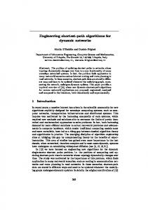
The lower bound for SPT is derived from pathological problem instances. It is quite likely that it actually does much better in practice. We would like to show this via experimentation. For this purpose, we used Python to implement SPT and another algorithm referred to as BASIC later. BASIC constructs a depth first search tree and then uses batch processing to send sensor readings along the tree to the sink. BASIC has been used in many real world sensor network deployment such as [15]. We also computed the three lower bounds on the number of hops given a network topology for comparison. They are: LB1: The number of non-sink vertices |V |, P LB2: v∈V d(v)/k, where d(v) is the smallest number of hops between v and the sink, and PD LB3: i=1 ni /k, where D is the distance from the sink to the vertex farthest away from the sink and ni is the number of vertices in G whose distance from the sink is at least i. The following parameters are varied to mimic different network scenarios: network topology, network size, network density, and k values. Figure 7 shows the impact of network size, node density and k value where sensor nodes 11

Figure 7: Performance of SPT in random topology: average ratio of the number of hops for SPT over the lower bound is 1.45, 1.29, and 1.14 for the three figures respectively. are uniformly randomly deployed in the network. We have omitted the results for grid topologies as similar trends were observed. In these figures, we only showed the maximum of the three lower bounds for comparison. (1) As the network size increases, the number of hops needed increases almost exponentially when BASIC is used but only increases moderately when SPT is used. This is because BASIC uses depth first search method to build the collection tree and the tree height increases as the network size or increases. (2) The number of hops for SPT decreases slightly as density increases, since the connectedness of the graph increases with density and this can decrease the depth of the tree. (3) When more readings can be included in one packet, the number of hops needed decreases when either algorithm is used, especially for BASIC. However, the performance of BASIC is still worse than the performance of SPT . The number of hops needed when SPT is used is only slightly higher than the lower bound in all cases, which validates our claim that SPT works well in practice. In all cases, the ratio of the number of hops for SPT over the lower bound is less than 1.5. Acknowledgement: We are thankful to M. V. Panduranga Rao and Dilys Thomas for participating in many discussions and providing valuable suggestions.

References [1] K. Akkaya and M. Younis. A survey of routing protocols for wireless sensor networks. Elsevier Ad Hoc Network Journal, 3(3):325–349, 2005. [2] Moses Charikar, Samir Khuller, and Balaji Raghavachari. Algorithms for capacitated vehicle routing. SIAM J. Comput., 31(3):665–682, 2001. [3] G. B. Dantzig and J. H. Ramser. The Truck Dispatching Problem. Management Science, 6(1):80–91, 1959. [4] Jr. E. G. Coffman, M. R. Garey, and D. S. Johnson. Approximation algorithms for bin packing: a survey, pages 46–93. PWS Publishing Co., Boston, MA, USA, 1997. [5] S. R. Gandham, Y. Zhang, and Q. Huang. Method and apparatus for optimizing convergecast operations in a wireless sensor network. U. S. Patent Office, June 2007. U.S. Patent Application Number 20070140149. [6] Michael R. Garey and David S. Johnson. Computers and intractability. Freeman, 1979. [7] A. Goel and D. Estrin. Simultaneous optimization for concave costs: single sink aggregation or single source buy-at-bulk. In Proceedings of ACM-SIAM Symposium on Discrete Algorithms (SODA), 2003. [8] W. R. Heinzelman, A. Chandrakasan, and H. Balakrishnan. Energy-efficient communication protocol for wireless microsensor networks. In Proceedings of Hawaii International Conference on System Sciences (HICSS), 2000.

12

[9] Barbara Hohlt, Lance Doherty, and Eric Brewer. Flexible power scheduling for sensor networks. In IPSN ’04: Proceedings of the 3rd international symposium on Information processing in sensor networks, pages 205–214, New York, NY, USA, 2004. ACM. [10] Bhaskar Krishnamachari, Deborah Estrin, and Stephen B. Wicker. The impact of data aggregation in wireless sensor networks. In ICDCSW ’02: Proceedings of the 22nd International Conference on Distributed Computing Systems, pages 575–578, Washington, DC, USA, 2002. IEEE Computer Society. [11] Stephanie Lindsey, Cauligi Raghavendra, and Krishna M. Sivalingam. Data gathering algorithms in sensor networks using energy metrics. IEEE Trans. Parallel Distrib. Syst., 13(9):924–935, 2002. [12] G. Lu, B. Krishnamachari, and C. S. Raghavendra. An adaptive energy-efficient and low-latency mac for treebased data gathering in sensor networks: Research articles. Wirel. Commun. Mob. Comput., 7(7):863–875, 2007. [13] M. Pan and Y. Tseng. Quick convergecast in zigbee beacon-enabled tree-based wireless sensor networks. Comput. Commun., 31(5):999–1011, 2008. [14] L. Paradis and Q. Han. Tigra: Timely sensor data collection using distributed graph coloring. In PERCOM ’08: Proceedings of the 2008 Sixth Annual IEEE International Conference on Pervasive Computing and Communications, pages 264–268, Washington, DC, USA, 2008. IEEE Computer Society. [15] L. Porta, T. H. Illangasekare, P. Loden, Q. Han, and A. P. Jayasumana. Continuous plume monitoring using wireless sensors: Proof of concept in intermediate scale tank. ASCE’s Journal of Environmental Engineering, 2009. To appear. [16] Paolo Toth and Daniele Vigo, editors. The vehicle routing problem. Society for Industrial and Applied Mathematics, Philadelphia, PA, USA, 2001. [17] S. Upadhyayula and S. K. S. Gupta. Spanning tree based algorithms for low latency and energy efficient data aggregation enhanced convergecast (dac) in wireless sensor networks. Ad Hoc Netw., 5(5):626–648, 2007. [18] Y. Yu and V. K. Prasanna. Energy-balanced task allocation for collaborative processing in wireless sensor networks. Mob. Netw. Appl., 10(1-2):115–131, 2005. [19] Ying Zhang, Shashidhar Gandham, and Qingfeng Huang. Distributed minimal time convergecast scheduling for small or sparse data sources. Real-Time Systems Symposium, IEEE International, 0:301–310, 2007.

13