Improved Sum-Min Decoding of Irregular LDPC Codes using

IMPROVED SUM-MIN DECODING OF IRREGULAR LDPC CODES USING NONLINEAR POST-PROCESSING Gottfried Lechner, and Jossy Sayir Telecommunications Research Center Vienna (ftw.) Donaucitystrasse 1/3, 1220 Vienna, Austria Email: {lechner|sayir}@ftw.at

ABSTRACT A novel method for improving the sum-min approximation for irregular low-density parity-check (LDPC) codes is presented. In comparison to previously published methods where the post-processing function has to change for every iteration, the new method allows the use of a fixed postprocessing function that can easily be implemented in practical system. Using this approach, the required signal to noise ratio is increased by only 0.15dB compared to the SumProduct decoder while keeping the implementation complexity low. 1. INTRODUCTION When implementing a decoder for low-density parity-check (LDPC) codes, the Sum-Product Algorithm (SPA) is often replaced by its approximation known as Sum-Min Algorithm (SMA). It has been recognized that the loss in performance due to this approximation, can be compensated by means of post-processing, i.e. performing a transformation of the output of the approximated check node function. The first analysis of post-processing was presented in [1, 2] where the authors proposed to apply a scaling factor or to subtract an offset of the check node output where the best values where found using density evolution. In [3], we presented an analytical derivation of the postprocessing function which turns out to be a nonlinear function and depends on various parameters. For regular codes, it has been shown in [3] that this nonlinear function can be well approximated by a scaling factor or an offset, confirming the heuristic approaches already presented in [1, 2]. For this approximation, two properties of regular LDPC codes are significant. First, all messages from variable to check nodes have the same distribution and second, the extrinsic information transfer (EXIT) curves of regular LDPC codes touch each other only in a single point in general. Therefore, it is sufficient to optimize the post-processing function for this single point. When applying the concept of post-processing to irregular LDPC codes, these two properties cease to apply. Messages from variable nodes of different degrees have different distributions. The optimal post-processing function, which depends on the distributions of those messages, is unpractical to compute for randomly constructed codes 1 . Furthermore, we showed in [5] that it is not sufficient to optimize the This work was partly supported by the European network of excellence NEWCOM. ftw. is a research institution within the Austrian competence center funding program Kplus. 1 It would be possible to compute this post-processing function for the case where the code has some structure as for example in [4], but this is not the focus of the present paper.

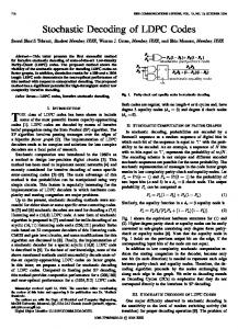
post-processing function for a single point in the EXIT chart, since the curves of variable and check node decoder touch each other almost everywhere if the degree distributions of the code are optimized in order to achieve capacity. In [5], we presented a method to apply post-processing sucessfully for irregular codes. The key element is to vary the post-processing function (which was approximated with a scaling factor) during the iterative decoding process resulting in a sequence of scaling factors compared to a single scaling factor for regular codes.2 A single scaling factor can easily be implemented in hardware using a lookup table. However, applying a varying scaling factor would require a new lookup table for every iteration, which is not convenient. In this work, we present a method which achieves the same (or even better) performance as varying scaling factors, but requires only a constant post-processing function that can easily be implemented in practical systems. We begin in Section 2 by reviewing the basics of postprocessing. In Section 3, we give an overview of approximations of the varying and nonlinear post-processing function and discuss their application to regular and irregular LDPC codes. The novel approach of using a constant, nonlinear function is presented in Section 4 and simulation results are presented in Section 5. 2. REVIEW OF POST-PROCESSING In this section, we review the derivation of the postprocessing function similar to [3, 5]. Let us first look at the model for computing the outgoing message of a check node when using the Sum-Product algorithm. The situation we are looking at, is shown in Figure 1. Given that dc binary variables fullfil a parity check equation, we aim to compute the L-value of one binary variable given the L-values of the dc − 1 other variables, where the received L-values are the output of binary input, symmetric output, memoryless channels with capacity Iai . It is well known that the solution for this problem is given by Ldc (L1 , . . . , Ldc −1 ) = 2 tanh−1

dc −1

Li

∏ tanh 2 . i=1

For the sum-min approximation we can state a similar problem depicted in Figure 2. Instead of observing dc − 1 Lvalues we have to compute the L-value of the desired variable 2 Another approximation of post-processing for irregular codes is presented in [6], where the authors applied normalization or offset to variable and check nodes depending on their degree.

parity check x1

ch1

x2

ch2

3. APPROXIMATIONS OF POST-PROCESSING

L1

3.1 Gaussian Approximation

L2

xdc −1

chdc −1

The first step in getting practical post-processing functions is to approximate the probability density functions of all incoming messages as being Gaussian with mean and variance depending only on the mutual information of the channels as

Ldc

SPA

Ldc −1

xd c

parity check x1

ch1

x2

ch2

L1 L2

xdc −1

chdc −1

Ldc −1

Z

SMA

Ldc

postprocessing

xd c

Figure 2: Model for check node operation using the SMA.

Using this approximation, we need to know the mutual information of all channels in order compute the desired L-value. For regular LDPC codes, we can assume that every channel has the same mutual information and therefore, the postprocessing function depends on a scalar value Ia only. For irregular codes, we make the approximation that the postprocessing function depends on the average mutual information of the channels. Applying this approximation, we get a post-processing function that is not parametrized by the probability density functions of the incoming messages but only by a scalar quantity.

given the output of the check node approximation Z written as dc −1

dc −1

i=1

i=1

Z (L1 , . . . , Ldc −1 ) = min |Li | ·

∏ sign(Li ) .

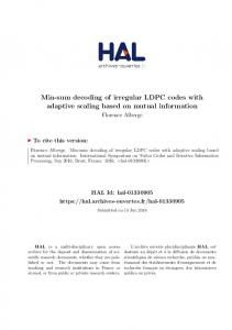
f (z; dc , p(·)) → f (z; dc , Ia ) Examples for this post-processing function are shown in Figure 3 for dc = 6 and several values of Ia . It can be ob-

We are still able to compute the L-value

10 I =0.5

Pr(Xdc = 0|Z = z) Ldc (z) = log Pr(Xdc = 1|Z = z)

a

φi− (ζ ) =

I a =0.99 6

4

2

Z +∞

pi (y)dy

Z −|ζ |

pi (y)dy.

L

+|ζ |

−∞

I a =0.75

8

as a function of Z analytically. Let pi (ζ ) denote the probability density function of Li and let φi+ (ζ ) and φi− (ζ ) be defined as the tail integrals

φi+ (ζ ) =

σi2 . 2

σi = J −1 (Ia,i ) and µi =

Figure 1: Model for check node operation using the SPA.

0

−2

−4

We can then write the L-value of our desired variable as Ldc (z) = f (z; dc , p(·)) = log

Ψ+ (z; dc , p(·)) , Ψ− (z; dc , p(·))

−6

(1)

where

−8

−10 −10

−8

−6

−4

−2

Ψ± (z; dc , p(·)) = dc −1

∑

dc −1

[pi (z) + pi (−z)]

i=1

∏

j=1; j6=i dc −1

± [pi (z) − pi (−z)]

[φi+ (z) + φi− (z)]

∏

j=1; j6=i

!

[φi+ (z) − φi− (z)] ,

and p(·) is a shorthand notation for the set of all dc −1 probability density functions of the incoming messages. Although the L-value of our desired variable node can be computed analytically, the computation requires the knowledge of the distributions of all incoming messages. In the next section we will show how these requirements can be relaxed in order to get practical post-processing functions.

0 Z

2

4

6

8

10

Figure 3: post-processing with Gaussian Approximation. served that, for large values of Ia , the post-processing function becomes an identity function. This is expected, since the sum-min approximation becomes more and more accurate for large values. 3.2 Linear Approximation The resulting post-processing function is still nonlinear and the dependency on the mutual information means that it has to be recomputed for every iteration. In [3], we showed how this function can be approximated by a linear function, where the approximation takes the probability density function of

the minimum Z into account. We define α (dc , Ia ) as the scaling factor which minimizes the expected squared error as

α (dc , Ia ) = argmin α0

Z ∞h −∞

f (z; dc , Ia ) − α 0 z

i2

15

10

· pZ (z; dc , Ia )dz. 5

Using this linear approximation, Equation 1 becomes

0

L

Ldc (z) = α (dc , IAc ) · z. 3.3 Optimization for the critical point

4. FIXED NONLINEAR POST-PROCESSING

−5

−10

−15 −15

−10

−5

0 Z

5

10

15

−10

−5

0 Z

5

10

15

1 0.9 0.8 0.7 0.6 pZ

After applying the linear approximation, we can further simplify the post-processing function by choosing the scaling factor that is most critical, i.e. the scaling factor where the tunnel between the EXIT curves is most narrow. For regular LDPC codes, where the curves touch each other only at a single point in general, this results in a scaling factor that can be kept constant over the iterations [3]. However, for irregular codes, where the curves fit each other tightly, this approximation can not be applied without a significant loss in performance. Therefore, for irregular LDPC codes we have to change the scaling factor from iteration to iteration, making it necessary for the decoder to store and apply a sequence of scaling factors. For details regarding this sequence of scaling factors, we refer to [5].

0.5 0.4

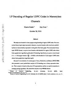
When implementing an LDPC decoder in hardware, a scaling factor can easily be applied by using a lookup table and thus avoiding the need for a multiplication. However, the application of a sequence of scaling factors would require either a new lookup table for every iteration, or a multiplication unit. Both options are not convenient for small and fast architectures. Therefore, we aim to apply a post-processing function that can be kept constant over the iterations without loss in performance, i.e. degradation of the threshold. We will demonstrate the basic idea with a simple example. Let us apply the Gaussian approximation of Section 3.1 for a check node of degree dc = 9. Figure 4 shows the postprocessing function and the probability density function of Z for Ia = 0.5 (solid lines) and for Ia = 0.99 (dashed lines). It can be observed, that the probability density function of Z for Ia = 0.5 has no significant contribution at magnitudes of Z larger than three. Therefore, the values of the postprocessing function above this magnitude are irrelevant when applying the post-processing function for Ia = 0.5. On the other hand, for a large value of Ia , the shape of the postprocessing function at small magnitudes has nearly no influence. We therefore propose to apply an universal, nonlinear post-processing function that is derived as a combination of post-processing functions weighted with the probability density function of the output of the sum-min approximation. We use a heuristic method to compute this universal postprocessing function. The universal post-processing function is computed as the weighted average between the minimum and the maximum Ia at the check node input as fA (z; dc) =

Z Ia,max Ia,min

f (z; dc , Ia ) · pZ (z; dc , Ia )dIa .

0.3 0.2 0.1 0 −15

Figure 4: post-processing function and probability density function of Z. 5. SIMULATION RESULTS In order to compare the results with previous publications, we used an irregular code with the same parameters as in [5]. The code is check regular with dc = 9 and the variable node distribution (edge perspective) is shown in the following table: degree 2 3 5 6 7 8 9 10 20 30

λ 0.212364 0.198528 0.008380 0.074687 0.014241 0.166518 0.009124 0.020019 0.000251 0.295888

The resulting rate is R = 0.5 and we set the block length to N = 105 in order to minimize the effects that are caused by cycles in the graph. The code was constructed using the progressive edge growth algorithm [7, 8].

In Figure 5, we show the universal post-processing function where we set Ia,min = 0.5 and Ia,max = 1.0. For comparison, we also show the post-processing functions for a single Ia at 0.5 and 0.99. It can be observed that for small magnitudes of Z, the universal function is close to the function for Ia = 0.5 and for large magnitudes the universal function gets close to the post-processing function for Ia = 0.99. This 10 universal I a =0.5

8

I =0.99 a

6

6. CONCLUSION We derived an universal post-processing function to improve the performance of the sum-min algorithm for decoding LDPC codes. While methods proposed in earlier publications require post-processing that varies over the number of iterations, we proposed a novel method that uses a constant post-processing function, that can easily be implemented using a lookup table. The needed variation of the post-processing over the iterations is achieved automatically by taking advantage of the properties of the sum-min output. The results were compared with previously published work and the new method outperforms previous methods while still being easier to implement.

4

REFERENCES

2

L

0

−2

−4

−6

−8

−10 −10

−8

−6

−4

−2

0 Z

2

4

6

8

10

Figure 5: Universal post-processing function. universal post-processing function is kept constant over the iterations and, using a maximum of 100 iterations, we obtain the bit error rates as shown in Figure 6. As a comparison, we included the curves for the sum-product algorithm, the summin algorithm without post-processing and the sum-min algorithm with varying scaling factors as presented in [5]. It can be observed that the universal post-processing function has the closest gap to the optimal sum-product algorithm and that the performance is very close to that of varying scaling factors. 10

0

SPA SMA variable scaling universal 10

−2

bit error rate

10

−1

10

10

−3

−4

0.5

1

1.5 E b/N0 [dB]

Figure 6: Bit error rates for proposed post-processing.

2

[1] Jinghu Chen and Marc P. C. Fossorier, “Near optimum universal belief propagation based decoding of low-density parity check codes,” IEEE Transactions on Communications, vol. 50, no. 3, pp. 406–414, March 2002. [2] Jinghu Chen and Marc P. C. Fossorier, “Density evolution for two improved BP-based decoding algorithms of LDPC codes,” IEEE Communications Letters, vol. 6, no. 5, pp. 208–210, May 2002. [3] G. Lechner and J. Sayir, “Improved sum-min decoding of LDPC codes,” in Proc. ISITA 2004, International Symposium on Information Theory and its Applications, Parma, Italy, 2004. [4] M. Fossorier and N. Miladinovic, “Irregular LDPC codes as concatenation of regular LDPC codes,” IEEE Communications Letters, vol. 9, no. 7, pp. 628–630, July 2005. [5] G. Lechner and J. Sayir, “Improved sum-min decoding for irregular LDPC codes,” in Proc. 4th International Symposium on Turbo Codes and Related Topics, Munich, Germany, 2006. [6] J. Zhang, M. Fossorier, and D. Gu, “Two-dimensional correction for min-sum decoding of irregular LDPC codes,” IEEE Communications Letters, vol. 10, pp. 180– 182, March 2006. [7] Xiao-Yu Hu, E. Eleftheriou, and D.M. Arnold, “Regular and irregular progressive edge-growth tanner graphs,” IEEE Transactions on Information Theory, vol. 51, no. 1, pp. 386–398, Jan 2005. [8] Xiao-Yu Hu, “Software for PEG code construction,” available at http://www.inference.phy.cam.ac.uk.