Proceedings of the 2004 IEEE International Conference on Robotics & Automation New Orleans, LA • April 2004
Improvements in robust 2D visual servoing ´ Eric Marchand, Andrew Comport, Franc¸ois Chaumette IRISA - INRIA Rennes Campus de Beaulieu, 35042 Rennes Cedex, France E-Mail:
[email protected] Abstract— A fundamental step towards broadening the use + Joint ∆ v P of real world image-based visual servoing is to deal with the s∗ cs + −λL Controler important issues of reliability and robustness. In order to address this issue, a closed loop control law is proposed that simultaneously accomplishes a visual servoing task and is robust s Extract features and reject outliers to a general class of image processing errors. This is achieved with Robust the application of widely accepted statistical techniques of robust M-estimation. Furthermore improvement have been added in the weight computation process: memory, initialization. Indeed, when Weights D Robust the error between current visual features and desired ones are depend on ∆ large, which occurs when large robot displacement are required, v M-estimator may not detect outliers. To address this point, the ∗ + P ∆ s Joint bL cs )+ D −λ(D method we propose to initialize the confidence in each feature Controler is based on the LMedS estimators. Experimental results are presented which demonstrate visual servoing tasks which resist s severe outlier contamination. Extract Features
I. I NTRODUCTION Visual servoing is targeted at controlling the movement of robotic systems by exploiting image sensor information. A general task being to move an end-effector to a certain pose with respect to particular objects or features in the image. This is known to be a very efficient method for positioning tasks [6]. However, its efficiency is subject to varying degrees of error. The efficiency of visual servoing relies on correspondences between the position of tracked visual features in the current image and their desired positions in the desired image. These correspondences are typically exploited in the form of a image error to be minimized. If these correspondences contain errors then visual servoing usually fails or convergences upon an imprecise position. Other sources of errors include those introduced by local detection and matching of features between the current and desired images. Overcoming this class of error is often achieved by improving the quality of tracking algorithms [11], [7], [1] and feature selection methods [9]. These approaches provide a robust input estimate to a control loop and as such treats outlier rejection, in an image processing step, prior to the visual servoing task (see Figure 1a). It is clear that handling all the potential sources of error by analytical classification is a very complex and difficult task. In this paper the problem of statistically robust visual servoing is implemented directly at a transient control law level (see Figure 1b). In order to represent all the possible external sources of error the correspondences may contain, a statistical measure of position uncertainty is sought. Let us note here that this paper is a sequel of a recent [2]. In this initial paper robust M-estimators [5] are employed
0-7803-8232-3/04/$17.00 ©2004 IEEE
(a)
(b)
Fig. 1. (a) Traditional outlier rejection (b) New proposed control law (see Section II-B for details)
because they give a solid statistical basis for detailed analysis and have even been considered to be a unifying banner for these estimation techniques [8]. The estimation of the standard deviation of the inlier data (scale) using the Median Absolute Deviation (MAD) means that no tuning is required. Furthermore, formulation in terms of an Iteratively Re-weighted Least Square (IRLS) allows simple integration directly into the visual control law. We had presented the details of the control law (including stability results) and compared various M-estimators (Huber, Cauchy, Tukey). Experimental results were presented on both simple images to show the validity of the control law and real images where points (detected using a Harris detector) were tracked using SSD trackers. However, though results were satisfactory a problem remains at the beginning of the positioning task when the error between current and desired position of the visual feature are large. In that case, outliers may not be detected and the robot trajectory may not be perfectly adequate. We address this problem in this paper using a LMedS-like method [10]. In addition we also consider a memory process on the weights in order to smooth the trajectory. New results will be presented. Following an introduction to the method, a robust control scheme is recalled in Section II-B. This is achieved by introducing a weight matrix in the error minimization. We present, in Section II-C how to use M-estimators to compute the weights which reflect a confidence in each feature in the image. In Section II-D, a new method to initialized weights
745
based on the LMedS approach is presented and finally in Section II-E we show how to combine both techniques to obtain satisfactory camera trajectory. Experimental results are presented in Section III. II. ROBUST V ISUAL S ERVOING
B. Robust Control Law The objective of the control scheme is to minimize the objective function given in equation (2). This new objective is incorporated into the control law in the form of a weight, which is given to specify a confidence in each feature location. Thus, the error to be minimized is given by: e = D(s(r) − s∗ ),
A. Overview and motivations The goal of classical visual servoing [3], [6] is essentially to minimize the error ∆ between a set of image features s(r), that depends of the camera pose r, and a set of desired image features s∗ : ∆ = s(r) − s∗ .
(1)
The camera then has to reach the pose rd that minimizes this error. However, as stated in the previous section, considering that s(r) is computed (from the image) with a sufficient accuracy is an important assumption. The control law that performs ∆ minimization is usually handled using a least square approach [3], [6]. However when the data contains outliers, such a classical approach is no longer efficient. A solution to handle this problem is to perform a robust minimization. M-estimators can be considered as a more general form of Maximum Likelihood Estimators (MLE) [5] because they permit the use of different minimization functions not necessarily corresponding to normally distributed data. Many functions have been presented in the literature which allow uncertain measures to be less likely considered and in some cases completely rejected. In the following subsections ρ is the objective function considered. The metric function to be minimized is modified to reduce the sensitivity to outliers. The robust optimization problem is then given by: ³ ´ ∆R = ρ s(r) − s∗ (2) where ρ(u) is a robust function [5] that grows subquadratically and is monotonically nondecreasing with increasing |u|. Considering a robust minimization will allow to compute the confidence in each feature. However this confidence is a statistic that depend only on the error s(r) − s∗ . When this error is large it may be difficult to detect outliers. Indeed, the error ∆i = si + ²i − s∗i (where ²i is an “aberration” due to imprecision in data extraction) is not statistically significant wrt. to the other errors ∆j . Since such important errors occurs mainly at the beginning of the positioning task is necessary at this point to provide a good initialization of the confidence in each feature. To embed a robust minimization in visual servoing, a modification of the control law is required to allow outlier rejection. The new control law is given in the next subsection while the weight computation method is presented in Section IIC (M-estimators), II-D (LMedS-based initialization) and II-E (weights fusion).
(3)
where D is a diagonal weighting matrix given by D = diag(w1 , . . . , wk ) The computation of weights wi are described in the next subsections. A simple control law can be designed to try to ensure an exponential decoupled decrease of e around the desired position s∗ (see [2] for more details). We obtain the following control law given by (see Figure 1b): ¢ ¡ bL cs )+ D s(r) − s∗ , (4) v = −λ(D
b a chosen model for D where v is the camera velocity, D c and Ls is a model or an approximation of the real interaction matrix Ls related to s (Ls links the camera motion v to the velocity of s in the image: s˙ = Ls v [6], [3]). This matrix depends on the value of the image features s and their corresponding depth Zd in the scene. It is classic in visual servoing to consider a constant Jacobian using the desired depth Zd and the desired value of bL cs )+ the features s∗ . In our case we can similarly define (D as: bL cs )+ = L+ (s∗ , Zd ), (5) (D s
Let us note that in [2], we have demonstrated the local stability of such system around s∗ . Of course it is necessary to ensure that a sufficient number of features will not be rejected so that DLs is always of full rank (6 to control the 6 dof of the robot). In fact, redundant features have to be used in s and our approach can thus not be applied for position-based or 2D 1/2 visual servoing since only six features are used in these methods. C. Computing the weights The weights wi , which represent the different elements of the D matrix and reflect the confidence of each feature, are usually given by [5]: wi =
ψ(δi /σ) δi /σ
(6)
³ ´ ∂ρ¡δ /σ¢ i where ψ δi /σ = (ψ is the M-estimate and is also ∂r called the influence function) and δi is the normalized residue given by δi = ∆i − M ed(∆) (where M ed(∆) corresponds to the median value taken across all the residues). In [2] we considered two influence functions that exist in the literature: Huber’s monotone function and Tukey’s hard re-descending function [5]. We showed that, since Tukey’s function allows to completely reject outliers and gives them
746
a zero weight, it is more interesting in visual servoing so that detected outliers have no effect on the robot motion. The corresponding influence function is given by: ½ u(b2 − u2 )2 , if |u| ≤ b (7) ψ(u) = 0 , else where the proportionality factor for Tukey’s function is b = 4.6851 which represents 95% efficiency in the case of Gaussian Noise [4]. The standard deviation of the inlier data or scale σ which appears in (6) is a robust estimate of the standard deviation of the good data and is at the heart of the robustness of the function. In visual servoing this estimate of the scale can vary dramatically during convergence. To avoid defining the scale as a tuning variable we use a robust statistic: the Median Absolute Deviation (MAD), given by: σ b=
1 M edi (|δi − M edj (δj )|). Φ−1 (0.75)
The algorithm described below enables a robust detection of the outliers within the whole set of features. Given n features si , i = 1 . . . n: 1) draw m subsamples sJ , J = 1 . . . m of k independent visual features. The maximum number of subsamples is mmax = (nk ), therefore if n is large mmax may be very large and a Monte Carlo technique may be used to draw the m subsamples (see note below). 2) for each subsample J, we compute the camera velocity vJ according to: ∗ vJ = −L+ sJ (sJ − sJ )
3) For each vJ , we determine the median of square residuals, denoted MJ , with respect to the whole set of features, that is: ¢2 ¡ MJ = med Lsi vJ + (si − s∗i ) i=1...n
(8)
where Φ(.) is the cumulative normal distribution function and 1 Φ−1 (0.75) = 1.48 represents one standard deviation of the normal distribution. D. Weights initialization using the LMedS approach When error s − s∗ is large, typically at the beginning of the positioning task, the error due to a misstracking or to a matching problem may not be statistically significant wrt. the expected error. In that case, if some outliers are not detected as such, corresponding weights are not equal to zero and the robot trajectory can be strongly perturbed. Therefore it is important to detect the points that are likely to be outliers prior the beginning of the servo process and to initialize adequately the weights. The Least-Median-of-Squares (LMedS) [10] method estimates the parameters by solving the non-linear minimization problem: min med ri2 i=1,...n
where ri is the residual for each available measure and n is the number of measure. In our case the camera velocity v is obtained by solving the following linear system: Ls v = −(s − s∗ ), the residual ri is given by: ¢2 ¡ ri2 = Lsi v + (si − s∗i )
4) We retain the value M ∗ that is minimal among all m MJ ’s. The corresponding vJ could be also of interest to control the robot, but we prefer to use a weighted control as described in Section II-B for such purpose1 . M ∗ will now be used to detect outliers. LMedS must be carefully designed to detect and remove outliers. Rousseeuw [10] proposes to assign a binary weight to each feature according to: ½ 1 if |ri | ≤ 2.5b σ wi = (9) 0 else where σ b is (as in eq (8)) a scale estimate defined by the robust statistic given by (see [10] for details): √ (10) σ b = 1.4826(1 + 5/(n − k)) M ∗
Note dealing with an important number of data: When n increases the number of possible subsamples increases drastically. Assuming that the whole set of features contains up to ε outliers (e.g., ε = 50%), the probability that at least one of the m subsamples contains only inliers is given by [10]: P = 1 − [1 − (1 − ε)k ]m If we require a good probability of detection (P ' 1), m can be computed given P , m and ε: m=
s∗i
are, respectively, the i-th line of the where Lsi , si and interaction matrix Ls and of the vector s and s∗ . Unlike M-estimators, the LMedS method cannot be reduced to a weighted least squares problem (and this is why we do not use it inside the control law but only for the initialization) and cannot be solved analytically. It must be solved by a search in the space of possible estimates generated from the data. This space is usually very large. In our case if we have n independent visual features its size is given by (nk ) where k is the minimal number of features that allows to perform a positionning task (6 ≤ k < n).
log(1 − P ) log[1 − (1 − ε)k ]
For example, when n¡ =¢20 and k = 6 an exhaustive search leads to mmax = 20 = 38760 subsamples where as, 6 with P = 0.99 and ε = 50%, only 293 subsamples are required. These m sample can be drawned using a Monte Carlo technique. 1 This is due to two reasons. The former is related to the complexity of this algorithm in term of computation. The latter is due to the fact that, if v j is considered to control the manipulator, only k features are then considered regardless of the number of inliers. Data redundancy that usually improves the robustness wrt. image noise would not be considered
747
E. Full weights computation Though not very complex, the LMedS-based outliers rejection algorithm requires some processing time that is not yet compatible with a 25Hz loop. That is why we consider it only for initialization. If we denote w tukey the weights computed from (6) and w LM edS the weights obtained from (9), a global weight can be defined as: wi = (1 − αt )witukey + αt wiLM edS
(11)
where α = 1 − exp(−β1 ks − s∗ k). When s − s∗ is large, α is close to 1 and only w LM edS are mainly considered. When the error s − s∗ decreases, it is easier and faster to detect outliers thanks to the M-estimator and weights w tukey are considered. Furthermore to smooth the weight evolution (and then the camera trajectory) it is also possible to introduce a memory process: wi0 (t) = β2 wi (t) + (1 − β2 )wi (t − 1)
(12)
with β2 ∈ [0 : 1] has to be tuned (1 if only the last computed weight wi (t) has to be considered). III. E XPERIMENTAL RESULTS The complete implementation of the robust visual servoing task, including tracking and control, was carried out on an experimental test-bed involving a CCD camera mounted on the end effector of a six d.o.f robot. We have considered positioning tasks. From an initial position, the robot has to reach a desired position expressed as a desired position of the object in the image. a) Visual features and weights computation: Some simple visual servoing experiments are considered that are based on the tracking of a pattern made with twelve white dots. Tracking such a simple pattern allows to validate the efficiency of the new control law. Indeed due to this simplicity, if no noise is artificially introduced in the point matching or in the tracking, a “control-case” is then available. Let us recall that our approach requires some redundancy in image data therefore multiple points (12 in the reported experiments) are extracted in the images. If n points are considered, s is a vector defined as s = (x1 , y1 , x2 , y2 , . . . , xn , yn ) where (xi , yi ) are the coordinates of the i − th point. Interaction matrix Ls is a 2n× 6 matrix given by Ls = (Ls1 , . . . , Lsn ) with: ¶ µ xi 0 x i yi −(1 + x2i ) yi − Z1i Z i Lsi = −xi yi −xi 0 − Z1i Zyii 1 + yi2 Weights are computed using equation (12) where ½ ∆2k = xk − xkd ∀k = 1 . . . n, ∆2k+1 = yk − ykd Since weights w2k and w2k+1 reflect the confidence we have in the same point, we define elements of the weights matrix D as D2k,2k = D2k+1,2k+1 = min(w2k , w2k+1 ).
b) Experiments: In these experiments, we considered our new visual servoing control law when large errors are introduced (other experiments are reported in [2]). Four experiments have been carried out: • [Exp 1] a reference experiment: a classical visual servoing task using the control law given in (4) with D = I ; • [Exp 2] an experiment with the same control law (still D = I, that is no robust estimation is considered) but artificial noise has been added in data extraction: an important error was introduced into the extracted coordinates of two points (points 0 and 2 on Figure 2 were voluntarily inverted) ; • [Exp 3] this experiment is similar to [Exp 2] but weights are computed as described by equation (6) using only Tukey M-estimator ; • [Exp 4] in this experiment we extend [Exp 3] by initializing weights using the new approach presented in section II-D ; As expected whereas the classical 2D visual servoing control law converges successfully toward the desired minimum when no error is introduced [Exp 1], a large error on two points [Exp 2] implies the convergence of the control law toward a local minimum. An error on the final coordinates of each point can be observed (see Figure 2c and plots on Figure 3 [Exp 2]), raw 2). Let us note that in some cases we can observe a complete divergence of the control law.
a
b
c
d
Fig. 2. Result of a positionning task using classical and robuste control law. On the image raw, first image show the initial camera position, the second shows the final camera position for the reference image, the third one shows the final camera view when no robust control law is considered (an error may be observed) and the later image shows the final camera view when the robust control law is considered).
Our new method improves the behavior of the positioning task. Indeed in the two other experiments where a weighting matrix is introduced in the control law [Exp 3-4] the camera reaches its final desired position with very good accuracy despite the errors introduced in the data. In [Exp 3] only Mestimator (Tukey) were considered in the weighting and the positioning precision is similar to the reference experiment (see Table I [Exp 3] vs [Exp 1]). We can note that at the
748
Camera velocity (translation)
Camera velocity (rotation)
0.035
error
0.05
Norm error ||we||
0.2
Vx Vy Vz
0.18
Rx Ry Rz
0.03
||we|| 0.16
0.04
0.15 0.14
0.025 0.03 0.1
0.12
0.02 0.02
0.1
0.015
0.05 0.08
0.01 0.01 0
0.06
0 0.005
0.04 -0.05
-0.01
0
0.02
-0.005
-0.02 0
100
200
300
400
500
600
700
800
900
1000
-0.1 0
100
200
300
400
500
600
700
800
900
1000
0 0
100
200
300
400
500
600
700
800
900
1000
0
100
200
300
400
500
600
700
800
900
1000
[Exp 1] Reference experiment (no error in the point matching) Camera velocity (translation)
Camera velocity (rotation)
0.035
error
0.05 Vx Vy Vz
0.03
0.025
Norm error ||we||
0.2
0.18
Rx Ry Rz
0.04
||we|| 0.16 0.15 0.14
0.03 0.1
0.02
0.12 0.02
0.015
0.05
0.1
0
0.08
0.01 0.01 0 0.005
0.06 -0.05 -0.01
0
0.04 -0.1
-0.02
-0.005
-0.01
0.02
-0.03 0
100
200
300
400
500
600
700
800
900
1000
-0.15 0
100
200
300
400
500
600
700
800
900
1000
0 0
100
200
300
400
500
600
700
800
900
1000
0
100
200
300
400
500
600
700
800
900
1000
[Exp 2] Classical control (an error is introduced in poitn matching) Camera velocity (translation)
Camera velocity (rotation)
0.035
error
0.04 Vx Vy Vz
Norm error ||we||
0.2
0.14
0.15
0.12
Rx Ry Rz
0.03
||we||
0.03
0.025 0.02
0.1
0.1
0.01
0.05
0.08
0.02
0.015 0
0
0.06
-0.01
-0.05
0.04
-0.02
-0.1
0.01
0.005
0
-0.005
-0.03 0
100
200
300
400
500
600
700
800
900
1000
0.02
-0.15 0
100
200
300
400
500
600
700
800
900
1000
0 0
100
200
300
400
500
600
700
800
900
1000
0
100
200
300
400
500
600
700
800
900
1000
[Exp 3] Robust control law considering only M-estimators Camera velocity (translation)
Camera velocity (rotation)
0.035
error
0.05 Vx Vy Vz
Norm error ||we||
0.2
0.12
0.15
0.1
Rx Ry Rz
0.03
||we||
0.04
0.025 0.03 0.1
0.08
0.05
0.06
0
0.04
0.02 0.02 0.015 0.01 0.01 0 0.005 -0.05
-0.01
0
-0.005
-0.02 0
100
200
300
400
500
600
700
800
900
1000
0.02
-0.1 0
100
200
300
400
500
600
700
800
900
1000
0 0
100
200
300
400
500
600
700
800
900
1000
0
100
200
300
400
500
600
700
800
900
1000
[Exp 4] Robust control law considering M-estimators and LMedS-based initialization Fig. 3. Result of a positioning task using classical and robust control laws. On each raw, plots depict from left to right the translational camera and rotational camera velocities, the errors si − s∗i for all the features and finally the weighted error kD(s − s∗ )k
no error large errors
Position reference no robust Mest tukey LMedS LMedS+Mest
[Exp 1] [Exp 2] [Exp 3] [Exp 4]
Tx -0,110 -127,337 -0,140 -0,133 -0,155
Ty -0,092 -102,909 -0,078 -0,211 0,072
Tz 0,026 29,873 -0,122 -0,185 -0,185
Rx -0,007 -3,140 -0,022 -0,018 -0,017
Ry -0,015 -15,629 -0,028 -0,052 -0,069
Rz 0,075 22,696 0,120 0,129 0,070
||T || 0,146 166,426 0,202 0,310 0,252
||R|| 0,077 27,735 0,126 0,140 0,100
TABLE I P OSITIONING ACCURACY SUMMARY: EACH LINE DISPLAYS THE ERROR ( IN CM AND DG ) BETWEEN THE DESIRED AND FINAL CAMERA POSITION .
beginning of the experiment, since all the error are large, as expected, the errors introduced in the point extraction si + δ − s∗i is not statistically significant wrt. the other errors si − s∗i and the values of the related weights are close to 1 at the beginning of the task (as can be seen on Figure 4a that shows the weights evolution). This leads to a discontinuous and noisy control law (see Figure 3 [Exp 3]). Furthermore the camera trajectory is very different from the “reference” trajectory (see Figure 5).
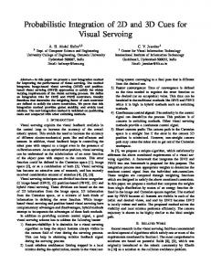
When the new weight initialization process is considered [Exp 4], it is possible to detect outliers before the beginning of the positioning task since it provides a better detection than the M-estimator for large error. However, if this approach is more efficient for large errors, when the errors decrease M-estimator should be considered. Indeed LMedS are very conservative and some inliers point may be considered as outliers (in this experiment two other points are initially considered as outliers). When the error decreases, M-estimators become more efficient and weight of outliers remains null while weight of inliers
749
Weights
extraction of the cog of another point. Despite these multiples errors and thanks to the robust control law, the expected minimum is reached.
1 w0 w2
0.8
0.6
0.4
0.2
a Fig. 6.
0
0
100
200
300
400
500
600
700
800
900
1000
b
c
Similar experiment but a 3D pattern is considered
a
Weights
IV. C ONCLUSION
1 w0 w2 w1 w11 0.8
0.6
0.4
0.2
0
0
100
200
300
400
500
600
700
800
900
1000
b
Fig. 4. Weights evolution for point detected as outliers (a) [Exp 3] only M-estimators (b) [Exp 5] LMedS and M-estimators. 0.5 reference [Exp 1] no robust [Exp 2] M−estimator [Exp 3] LMedS + M−estimator [Exp 5]
0.45
A novel visual servoing method has been proposed that rejects errors in feature extraction, tracking and matching at the transient control law level. To achieve this goal, a robust M-estimation was integrated directly via an iteratively re-weighted least squares method. Previous visual servoing methods have only considered outlier rejection in the image processing step. Extending the method proposed in [2], we considered the problem of weights initialization in order to detect earlier aberrant data. The resulting control is now more continuous and the robot trajectory is now similar to the reference trajectory (with no aberrant data). Experimental results show the efficiency of the approach for a positioning task on case-study examples for planar and non-planar objects. In both cases a great improvement in the positioning accuracy has been observed wrt. a non robust control law and a better trajectory is obtained wrt. the use of a robust control law considering only M-estimator as proposed in our earlier work.
0.4
R EFERENCES z
0.35
0.3
0.25
0.2 0.5 0 −0.5 −0.25 y
−0.2
−0.1
−0.15
−0.05
0
0.05
0.1
x
Fig. 5.
Camera trajectory for important matching errors.
tends toward 1 (see Figure 4b) since LMedS initialization is “forgotten” according to equation (11). As can be seen on Figure 4b, final weights of outliers are always close to zero which implies that the evolution of the camera velocity (see Figure 3 [Exp 1-4]) as well as its trajectory (on Figure 5) may favorably be compared with the reference experiment. In the last experiment (see Figure 6) we show that our approach does not depend on the target geometry and is also suitable for non-planar scene (here 18 non coplanar points have been used). In addition we also consider more outliers: two sets of points where inverted (see the blue lines on figure 6 and the white patch in the corner simulates an error in the
[1] A. Comport, E. Marchand, and F. Chaumette. A real-time tracker for markerless augmented reality. In ACM/IEEE Int. Symp. on Mixed and Augmented Reality, ISMAR’03, pages 36–45, Tokyo, Japan, October 2003. [2] A. Comport, M. Pressigout, E. Marchand, and F. Chaumette. A visual servoing control law that is robust to image outliers. In IEEE Int. Conf. on Intelligent Robots and Systems, IROS’03, volume 1, pages 492–497, Las Vegas, Nevada, October 2003. [3] B. Espiau, F. Chaumette, and P. Rives. A new approach to visual servoing in robotics. IEEE Trans. on Robotics and Automation, 8(3):313–326, June 1992. [4] P.-W. Holland and R.-E. Welsch. Robust regression using iteratively reweighted least-squares. Comm. Statist. Theory Methods, A6:813–827, 1977. [5] P.-J. Huber. Robust Statistics. Wiler, New York, 1981. [6] S. Hutchinson, G. Hager, and P. Corke. A tutorial on visual servo control. IEEE Trans. on Robotics and Automation, 12(5):651–670, October 1996. [7] D. Kragic and H. Christensen. Cue integration for visual servoing. IEEE Trans. on Robotics and Automation, 17(1):19–26, February 2001. [8] P. Meer, C. V. Stewart, and D. E. Tyler. Robust computer vision: An interdisciplinary challenge. Computer Vision and Image Understanding: CVIU, 78(1):1–7, 2000. [9] N. P. Papanikolopoulos and P. K Khosla. Selection of features and evaluation of visual measurements for 3-d robotic visual tracking. Int. Symp. on Intelligent Control., pages 320–325, August 1993. [10] P.J. Rousseeuw and A.M. Leroy. Robust Regression and Outlier Detection. John Wiley and Sons, New York, 1987. [11] T. Tommasini, A. Fusiello, E. Trucco, and V. Roberto. Making good features track better. In IEEE Int. Conf. on Computer Vision and Pattern Recognition, pages 178–183, Santa Barbara, USA, June 1998.
750