Therefore, we present a modelâ based system where a wireâframe model of the object is ...... http://www.nada.kth.se/cvap/cvaplop/lop-cvap.html,. January 2002.
Robust Visual Servoing D. Kragic and H. I. Christensen Centre for Autonomous Systems Computational Vision and Active Perception Royal Institute of Technology, SE–100 44 Stockholm, Sweden {danik,hic}@nada.kth.se ∗ Abstract For service robots operating in domestic environments it is not enough to consider only control level robustness - it is equally important to consider how image information that serves as input to the control process can be used so as to achieve robust and efficient control. This paper presents an effort towards development of robust visual techniques used to guide robots in various tasks. Given a task at hand, we argue that different levels of complexity should be considered which also defines the choice of the visual technique used to provide the necessary feedback information. We concentrate on visual feedback estimation where we investigate both two– and three– dimensional techniques. In the former case, we are interested in providing a coarse information about the object position/velocity in the image plane. In particular, a set of simple visual features (cues) is employed in an integrated framework where voting is used for fusing the responses from individual cues. The experimental evaluation shows the system performance for three different cases of camera–robot configurations most common for robotic systems. For cases where the robot is supposed to grasp the object, a two–dimensional position estimate is often not enough. Complete pose (position and orientation) of the object may be required. Therefore, we present a model– based system where a wire–frame model of the object is used to estimate its pose. Since a number of similar systems has been proposed in the literature, we concentrate on the particular part of the system usually neglected - automatic pose initialization. Finally, we show how a number of existing approaches can successfully be integrated in a system that is able to recognize and grasp fairly textured, everyday objects. One of the examples presented in the experimental section shows a mobile robot performing tasks in a real–word environment – a living room. ∗ This research has been sponsored by the Swedish Foundation for Strategic Research through the Centre for Autonomous Systems. The funding is gratefully acknowledged.
1 Introduction Robotics is gradually expanding its application domain beyond manufacturing. In manufacturing settings it is possible to engineer the environment so as to simplify detection and handling of objects. In an industrial context this is often achieved through careful selection of background color and lighting. As the application domain is expanded, the use of engineering to simplify the perception problem is becoming more difficult. It is not longer possible to assume a given setup of lighting and a homogeneous background. Recent progress in service robotics shows a need to equip robots with facilities for operation in everyday settings where the design of computer vision methods to facilitate robust operation and to enable interaction with objects have to be reconsidered. This paper considers the use of computational vision for manipulation of objects in everyday settings. The process of manipulation of objects involves all aspects of recognition/detection, servoing to the object, alignment and grasping. Each of these processes have typically been considered independently or in relatively simple environments, [1]. Through careful consideration of the task constraints and combination of multiple methods it is, however, possible to provide a system that exhibits robustness in realistic settings. The paper starts with a motivation that argues for integration of visual processes in Section 2. A key competence for robotic grasping is recognition/detection of objects as outlined in Section 3. Once the object has been detected, the reaching phase requires use of a coarse servoing strategy which can be based on “simple” visual features. Unfortunately, “simple” visual features suffer from a limited generality requiring therefore an integration of multiple cues to achieve robustness as described in Section 4. Once the object has been recognized and an approximate alignment has been achieved, it is possible to use model based methods for accurate interaction with the object as outlined in Section 5. Finally, all of these components are integrated into a complete system and used for a series of experiments. The
results from these experiments are presented and discussed in Section 6. The overall approach and the associated results are discussed in Section 7.
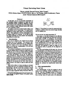
2 Motivation Robotic manipulation in an everyday setting is typically carried out in the context of a task such as “Please, fetch the cup from the dinner table in the living room.” or “Please, fetch the rice package from the shelf.”, (see Fig. 1). To execute such a manipulation task, we use a mobile platform with a manipulator on the top. The robot is equipped with facilities for automatic localization and navigation, [2] allowing it to arrive at a position in the vicinity of the dinner table. From there the robot is required to carry out the following: 1. Recognize a cup on the table (discussed in Section 3). 2. Transportation – servo to the vicinity of the cup, potentially involving both platform and manipulator motion (discussed in Section 4). 3. Estimate the pose (position and orientation) of the object (Section 5). 4. Alignment – servo to the object to allow grasping (Section 5). 5. Pick up the object and drive away.
Figure 1: An example of a robot task: Fetching a rice package from a shelve. In a typical scenario, the distance between the object and the on-board camera may vary significantly. This implies a significant uncertainty in terms of scale (i.e., size of
the object in the image). Based on the actual scale of the object in the image a hierarchical strategy for visual servoing may be used. For distant objects (≥ 1m), there is no point in attempting to perform a full pose estimation, as the size of the object in the image typically will not provide the necessary information. A coarse position estimate is therefore adequate for an initial alignment. A visual servoing task in general includes some form of i) positioning such as aligning the robot/gripper with the target, and ii) tracking – updating the position/pose of the image features/object. Typically, image information is used to measure the error between some current and reference/desired location. Image information used to perform the task is either i) two dimensional – using image plane coordinates, or ii) three dimensional – retrieving objects’ pose parameters with respect to the camera/world/robot coordinate system. So, the robot is controlled either using image information as two- or three dimensional which classifies the visual servoing approaches as i) image based, ii) position based or iii) hybrid visual servoing (2.5D servoing), [17]. If the object is far from the camera, due to the resolution/size of the object in the image, it is advantageous to use an image based strategy to perform the initial alignment. Image based servoing using crude image features such as center of mass is well suited for coarse alignment. A problem here is that visual cues such as color, edges, corners or fiducial marks in general are highly sensitive to variation in illumination, etc. and no single one of them will provide robust frame by frame estimates that allow continuous tracking. Through their integration is however possible to achieve an increased robustness as described in Section 4. For the accurate alignment of the gripper with the object one can utilize i) a binocular camera pair, ii) a monocular image in combination with a geometric model, or iii) one camera in combination with a “structure–from–motion” approach. As the object has been recognized and its approximate image position is known, it is possible to utilize this information for efficient pose estimation using a wire–frame model. Model based fitting is highly sensitive to surface texture and background noise. The availability of a good initial estimate does, however, allow robust estimation of pose even in the presence of significant noise. Once a pose estimate is available, it is possible to use 2.5D or position based servoing for the alignment of the gripper with the objects. This is even possible in the presence of significant perspective effects, which typically is the case when operating close to objects. Model based tracking is in general highly sensitive to surface texture and initialization, but through its integration into a system context these problems are reduced to a minimum as outlined in Sec-
tion 5. Finally, as the gripper is approaching the object it is essential to use the earlier mentioned geometric model for grasp planning, an issue not discussed in detail here. For an introduction consult [4], [26].
3 Detection and Pose Estimation Given a view of the scene, the robot should be able to find/recognize the object to be manipulated or give us an answer such as “I-did-not-find–the–cup”. This task is very complicated and hard to generalize with respect to cluttered environments and types of objects. Depending on the implementation, the recognition process may provide partial/full pose of the object which can in return be used for generating the robot control sequence. Object recognition is a long standing research issue in the field of computational vision [11]. We consider limited aspects of it, but demonstrate recognition in real environments, a problem that has received limited attention so far.
rice 1.09549 raisins 1.73754
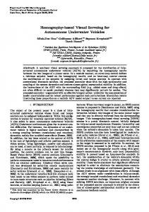
[23]. The objective here is to detect and recognize everyday household objects in a scene. The recognition step delivers the image position and approximate size of the image region occupied by the object, see Fig. 2. This information is in our case used to i) track the part of the image, the window of attention, occupied by the object while the robot approaches it, or ii) as the input to the pose estimation algorithm.
3.2 Feature Based Method In case of a moving object, its appearance may change significantly between frames. For that reason, we have also exploited a feature or a cue based method. Here, color and motion were used in an integrated framework where voting was used as an underlying integration strategy. This is discussed in more detail in the next section.
4 Transportation Coarse Visual Servoing While approaching the object, we want to keep in the field of view or even centered of the image. This implies that we have to estimate the position/velocity of the object in the image and use this information to control the mobile platform. Our tracking algorithm employs the four step detect– match–update–predict loop, Fig. 3. The objective here is to track a part of an image (a region) between frames. The image position of its center is denoted with p = [x y]T . Hence, the state is x = [ x y x˙ y˙ ]T where a piecewise constant white acceleration model is used [3]: xk+1 = Fxk + Gvk zk = Hxk + wk
Figure 2: An example where the recognition system successfully recognizes two of the objects. Above each rectangle there is a value representing the recognition confidence which is proportional to the distance of the object to the hyperplane of the classifier. In order to make confidence measures comparable across all the classifiers, the distances are normalized with the margin of the hyperplane of the classifier. If the confidence is greater than 1, a positive detection/recognition is assumed. If the confidence is less than 1, the classification is considered uncertain.
where vk is a zero–mean white acceleration sequence, wk is measurement noise and ∆T 2 � 1 0 ∆T 0 � 0 2 � � 0 ∆T 2 , H = 1 0 0 0 (2) F = 00 10 01 ∆T 0100 0 , G= 2 00 0
∆T 0
1
0 ∆T
For prediction and estimation, the α − β filter is used, [3]: xˆ k+1|k = Fk xˆ k zˆ k+1|k = Hˆxk+1|k
(3)
xˆ k+1|k+1 = xˆ k+1|k + W[zk+1 − zˆ k+1|k ]
3.1 Appearance Based Method with The object to be manipulated is recognized using the viewbased SVM (Support Vector Machine) system presented in
(1)
W=
�
β 0 α 0 ∆T β 0 α 0 ∆T
�T
where α and β are determined using steady–state analysis.
not found
Search
found
The cues considered in the integration process are: Correlation - The standard sum of squared differences (SSD) similarity metric is used and the position of the target is found as the one giving the lowest dissimilarity score:
Initialization
Exit
SSD(u, v) = ∑ ∑ [I(u + m, v + n) − T(m, n)]2
N
Detection
Y
Matching
^ x k+1|k ^zk+1|k
z k+1
Estimation
^x k+1|k+1
Figure 3: A schematic overview of the tracking system.
4.1 Voting Voting, in general, may be viewed as a method to deal with n input data objects, ci , having associated votes/weights wi (n input data–vote pairs (ci , wi )) and producing the output data–vote pair (y, v) where y may be one of the ci ’s or some mixed item. Hence, voting combines information from a number of sources and produces outputs which reflect the consensus of the information. The reliability of the results depends on the information carried by the inputs and, as we will see, their number. Although there are many voting schemes proposed in the literature, mean, majority and plurality voting are the most common ones. In terms of voting, a visual cue may be motion, color or disparity. Mathematically, a cue is formalized as a mapping from an action space, A, to the interval [0,1]: (4)
This mapping assigns a vote or a preference to each action a ∈ A, which may, in the context of tracking, be considered as the position of the target. These votes are used by a voter or a fusion center, δ(A). Based on the ideas proposed in [5], [24], we define the following voting scheme: Definition 4. 1 - Weighted Plurality Approval Voting For a group of homogeneous cues, C = {c1 , . . . , cn }, where n is the number of cues and Oci is the output of a cue i, a weighted plurality approval scheme is defined as: (5)
i=1
where the most appropriate action is selected according to: a0 = argmax{δ(a)|a ∈ A}
where I(u, v) and T (u, v) represent the grey level values of the image and the template, respectively. To compensate for changes in the appearance of the tracked region, the template is updated on 25 frames cycle. Color - It has been shown in [7] that efficient and robust results can be achieved using the Chromatic Color space. Chromatic colors, known as “pure” colors without brightness, are obtained by normalizing each of the components by the total sum. Color is represented by r and g component since blue component is both the noisiest channel and it is redundant after the normalization. Motion - Motion detection is based on computation of the temporal derivative and image is segmented into regions of motions and regions of inactivity. This is estimated using image differencing: M [(u, v), k] = H [|I [(u, v), k] − I [(u, v), k − 1]| − Γ] (8) where Γ is a fixed threshold and H is defined as: � 0 : x≤0 H (x) = x : x>0
(9)
Intensity Variation - In each frame, the following is estimated for all m × m (details about m are given in Section 4.4.2) regions inside the tracked window: σ2 =
1 ¯ v)]2 ∑ [I(u, v) − I(u, m2 ∑ u v
(10)
¯ v) is the mean intensity value estimated for the where I(u, window. For example, for a mainly uniform region, low variation is expected during tracking. On the other hand, if the region was rich in texture large variation is expected. The level of texture is evaluated as proposed in [25].
4.3 Weighting
n
δ(a) = ∑ wi Oci (a)
(7)
n m
Prediction
c : A → [0, 1]
4.2 Visual Cues
(6)
In (Eq. 5) it is defined that the outputs from individual cues should be weighted by wi . Consequently, the reliability of a cue should be estimated and its weight determined based on its ability to track the target. The reliability can be determined either i) a–priori and kept constant during tracking, or ii) estimated during tracking based on cue’s success to
estimate the final result or based on how much it is in agreement with other cues. In our previous work the following methods were evaluated [19]: 1. Uniform weights - Outputs of all cues are weighted equally: wi = 1/n, where n is the number of cues. 2. Texture based weighting - Weights are preset and depend on the spatial content of the region. For a highly textured region, we use: color (0.25), image differencing (0.3), correlation (0.25), intensity variation (0.2). For uniform regions, the weights are: color (0.45), image differencing (0.2), correlation (0.15), intensity variation (0.2). The weights were determined experimentally. 3. One-step distance weighting - Weighting factor, wi , of a cue, ci , at time step k depends on the distance from the predicted image position, zˆ k|k−1 . Initially, the distance is estimated as di = ||zik − zˆ k|k−1 ||
4.4 Implementation We have investigated two approaches where voting is used for: i) response fusion, and ii) action fusion. The first approach makes use of “raw” responses from the employed visual cues in the image which also represents the action space, A. Here, the response is represented either by a binary function (yes/no) answer, or in the interval [0,1] (these values are scaled between [0,255] to allow visual monitoring). The second approach uses a different action space represented by a direction and a speed, see Fig. 4. Compared to the first approach, where the position of the tracked region is estimated, this approach can be viewed as estimating its velocity. Again, each cue votes for different actions from the action space, A, which is now the velocity space. SPEED slow
(11) 4 left
and errors are estimated as
wait
6 down
ei =
di . n ∑i=1 di
DIRECTION
SPEED
fast up 2 0 right
wi
2wi
0 1 2 3 4 5 6 7
4wi 2wi wi
wait slow
fast
DIRECTION
(12) Figure 4: A schematic overview of the action fusion approach:
Weights are than inversely proportional to the error with ∑ni=1 wi = 1. 4. History-based distance weighting - Weighting factor of a cue depends on its overall performance during the tracking sequence. The performance is evaluated by observing how many times the cue was in an agreement with the rest of the cues. The following strategy is used: j
a) For each cue, ci , examine if ||zik − zk || < dT where i, j = 1, . . . , n and i 6= j. If this is true, ai j =1, otherwise ai j =0. Here, ai j =1 means that there is an agreement between the outputs of cues i and j at that voting cycle and dT represents a distance threshold which is set in advance. b) � Build the (n − 1) value set for each cue: ci : ai j | j = 1, . . . , n and i 6= j and estimate sum si = ∑nj=1 ai j . c) The accumulated values during N tracking cycles, Si = ∑Nk=1 ski , indicate how many times a cue, ci , was in the agreement with other cues. Weights are then simply proportional to this value:
the desired direction is (down and left) with a (slow) speed. The use of bins represents a neighborhood voting scheme which ensures that slight differences between different cues do not result in an unstable classification.
4.4.1 Initialization According to Fig. 3, a tracking sequence should be initiated by detecting the target object. If a recognition module is not available, another strategy can be used. In [28] it is proposed that selectors should be employed which are defined as heuristics that selects regions possibly occupied by the target. When the system does not have definite state information about the target it should actively search the state space to find it. Based on this ideas, color and image differences (or foreground motion) may be used to detect the target in the first image. Again, if a recognition module is not available, these two cues may also be used in cases where the target has either i) left the field of view, or ii) it was occluded for a few frames. Our system searches the whole image for the target and once the target enters the image, tracking is regained. 4.4.2 Response Fusion Approach
wi =
Si ∑ni=1 Si
n
with
∑ wi = 1
i=1
(13)
After the target is located, a template is initialized which is used by the correlation cue. In each frame, a color image
^ x k+1|k w1 w2
c1 c2
^zk+1|k
^x k+1|k+1
Prediction
O1
0 ≤ Ovar (x, k) ≤ 255 with x ∈ [ˆzk|k−1 − 0.5xw , zˆ k|k−1 + 0.5xw ]
O2
z k+1 VOTING
wn
cn
with n = 0.2xw . Hence, for a 30 × 30 pixels window of attention, m=6. The result is presented as follows:
Estimation
On
(17)
Response Fusion The estimated responses are integrated using (Eq. 5): n
δ(x, k) = ∑ wi Oi (x, k)
Detect/Match
(18)
i
Figure 5: A schematic overview of the response fusion approach. of the scene is acquired. Inside the window of attention the response of each cue, denoted Oi , is evaluated, see Fig. 5. Here, x represents a position: Color - During tracking, all pixels whose color falls in the pre–trained color cluster are given value between [0, 255] depending on the distance from the center of the cluster: 0 ≤ Ocolor (x, k) ≤ 255 with x ∈ [ˆzk|k−1 − 0.5xw , zˆ k|k−1 + 0.5xw ]
2 (− x¯2 ) 2σ
(15)
with σ = 5
x ∈ [zSSD − 0.5xw , zSSD + 0.5xw ], x¯∈ [−0.5xw , 0.5xw ]
0
1:
4.4.3 Action Fusion Approach
Correlation - Since the correlation cue produces a single position estimate, the output is given by:
OSSD (x, k) = 255e
0
if δ(x, k) is argmax{δ(x , k)|x δ (x, k) = ∈ [ˆzk|k−1 − 0.5xw , zˆ k|k−1 + 0.5xw ]} 0: otherwise (19) Finally, the new measurement zk is given by the mean value 0 0 (first moment) of δ (x, k), i.e., zk = δ¯(x, k). 0
(14)
where xw is the size of the window of attention. Motion- Using (Eq. 8) and (Eq. 9) with Γ = 10, image is segmented into regions of motion and inactivity: 0 ≤ Omotion (x, k) ≤ 255 − Γ with x ∈ [ˆzk|k−1 − 0.5xw , zˆ k|k−1 + 0.5xw ]
However, (Eq. 6) can not be directly used for selection, as there might be several pixels with same number of votes. Therefore, this equation is slightly modified:
(16)
where the maximum of the Gaussian is centered at the peak of the SSD surface. The size of the search area depends on the estimated velocity of the region. Intensity variation - The response of this cue is estimated according to (Eq. 10). If a low variation is expected, all pixels inside an m × m region are given values (255-σ). If a large variation is expected, pixels are assigned σ value directly. The size m×m of the subregions which are assigned same value depends on the size of the window of attention
Here, the action space is defined by a direction d and speed s, see Fig. 4. Both the direction and the speed are represented by histograms of discrete values where the direction is represented by eight values, see Fig. 6: � −1 � � 0 � � � � −1 � LD −1 1 , L 0 , LU −1 , U −1 , (20) � � � � � 1 � �1� RU −1 , R 0 , RD 11 , D 01
with L-left, R-right, D-down and U-up. Speed is represented by 20 values with 0.5 pixel interval which means that the maximum allowed displacement between successive frames is 10 pixels (this is easily made adaptive based on the estimated velocity). There are two reasons for choosing just eight values for the direction: i) if the update rate is high or the inter–frame motion is slow, this approach will still give a reasonable accuracy and hence, a smooth performance, and ii) by keeping the voting space rather small there is a higher chance that the cues will vote for the same action. Accordingly, each cue will vote for a desired direction and a desired speed. As presented in Fig. 4, a neighborhood voting scheme is used to ensure that slight differences between different cues do not result in an unstable classification. (Eq. 3) is modified so that: H=
�0 0 1 0� 0001
and W =
h
α∆T 0 β 0 0 α∆T 0 β
iT
(21)
In each frame, the following is estimated for each cue: Color - The response of the color cue is first estimated according to (Eq. 14) followed by: ∑x Ocolor (x, k)x(k) − pˆ k|k−1 ∑x x(k) with x ∈ [pˆ k|k−1 − 0.5xw , pˆ k|k−1 + 0.5xw ] acolor (k) =
^ x k+1|k w1 w2
(22)
^z k+1|k
Prediction
left c1 c2
right up down
where acolor (k) represents the desired action and pˆ k|k−1 is the predicted position of the tracked region. Same approach is used to obtain amotion (k) and avar (k). Correlation - The minimum of the SSD surface is used as:
^x k+1|k+1
VOTING
z k+1
Estimation
wait wn
fast cn
slow
Detect/Match
aSSD (k) = argmin(SSD(x, k)) − pˆ k|k−1
(23)
x
Figure 6: A schematic overview of the action fusion approach.
where the size of the search area depends on the estimated velocity of the tracked region. Action Fusion After the desired action, ai (k), for a cue is estimated, the cue produces the votes as follows: direction di = P (sgn(ai )), speed si = ||ai ||
(24)
where P : x → {0, 1, . . . , 7} is a scalar function that maps the two–dimensional direction vectors (see (Eq. 20)) to one–dimensional values representing the bins of the direction histogram. Now, the estimated direction, di , and the speed, si , of a cue, ci , with a weight, wi , are used to update the direction and speed of the histograms according to Fig. 4 and (Eq.5). The new measurement is then estimated by multiplying the actions from each histogram which received the maximum number of votes according to (Eq. 6): zk = S (argmax HD(d)) argmax HS(s) d
(25)
s
� � � −1 � where S : x → { −1 0 , . . . , 1 }. The update and prediction steps are then performed using (Eq. 21) and (Eq. 3). The reason for choosing this particular representation instead of simply using a weighted sum of first moments of the responses of all cues is, as it has been pointed out in [24], that arbitration via vector addition can result in commands which are not satisfactory to any of the contributing cues.
4.5 Examples The proposed methods have been investigated in detail in [19]. Here, we present one of the experiments where we evaluated the performance of the voting approaches as well as the performance of individual cues with respect to three sensor–object configurations typically used in visual–servoing systems: i) static sensor/moving object
(“stand–alone camera system”), ii) moving sensor/static object (“eye–in–hand camera” servoing toward a static object), and iii) moving sensor/moving object (camera system on a mobile platform or eye–in–hand camera servoing toward a moving object). The results are discussed through accuracy and reliability measures. The accuracy is expressed using an error measure which is a distance between the ground truth (chosen manually using a reference point on the object) and the currently estimated position of the reference point. The results are summarized through the mean square error and standard deviation in pixels. The measure of the reliability is on a yes/no basis depending on if a cue (or the fused system) successfully tracks the target during a single experiment. The tracking is successful if the object is kept inside the window of attention during the entire test sequence. The two fusion approaches as well as the individual cues have been tested with respect to the ability to cope with occlusions of the target and to regain tracking after the target has left the field of view for a number of frames. The results are presented for correlation, color and image differences since the intensity variation cue can not be used alone for tracking. Accuracy (Table 1) - As it can be seen from the table, the best accuracy is achieved using the response fusion approach. Although the mse is similar for the action fusion approach in cases of static sensor/moving object and moving sensor/static object configurations, std is higher. The reason for this is the choice of the underlying voting space. For example, if the color cue shows a stable performance for a number of frames, its weight will be high compared to the other cues (or it might have been set to a high value from the beginning). In some cases, like in the case of a box of raisins presented in Fig. 7, two colors are used at the same time. When an occlusion occurs, the position of the
Figure 7: Example images from a raisin package tracking. center of the mass of the color blob will change fast (and sometimes in different directions) which results in abrupt changes in both direction and speed. The other method, response fusion, on the other hand, does not suffer from this which results in a lower standard deviation value. The comparison of the performance of the fusion approaches and the performance of the individual cues shows the necessity for fusion. Image differences alone can not be used in cases of moving sensor/static object and moving sensor/moving object configurations since there is no ability to differ between the object and the background. As mentioned earlier, during most of the sequences the target undergoes 3D motion which results with scale changes and rotations not modeled by SSD. It is obvious that these factors will affect this cue significantly resulting with a large error as demonstrated in the table. This problem may be solved by using a better model (affine, quadratic, see [15]). It can also be seen that the color cue performed best of the individual cues. In the case of moving sensor/static object after the tracking is initialized the color cue “sticks” to the object during the sequence and, since the background varies a little, the best accuracy is achieved compared to other configurations. During other two configurations the background will change containing also the color same as the target’s. This distracts the color tracker resulting in increased error. The error is larger in the case of static sensor/moving object compared to moving sensor/moving object since in the test sequences the background included the target’s color more often. Reliability (Table 2) - The reliability is expressed through a number of successful runs where the accuracy is obtained using the texture based weighting. In Table 2, the obtained reliability results are ranked showing that color performs most reliably compared to other individual cues. In certain cases, especially when the influence of the background is not significant, this cue will perform satisfactorily. However, it will easily get distracted if the background takes a large portion of the window of attention and includes the target’s color. Image differencing will depend on the size of the moving target with respect to the size of the window of attention and variations in lighting. In
static sensor/
moving sensor/
moving sensor/
moving object
static object
moving object
mse
std
mse
std
mse
std
RF
7
7
4
3
9
10
AF
7
9
4
10
13
25
Color
15
16
10
6
10
14
Diff
23
26
failed
failed
failed
failed
SSD
25
27
12
13
17
21
Table 1: Qualitative results for various sensor-object configurations (in pixels).
structured environments, however, this cue may perform well and may be considered in cases of a single moving target where the size of the target is small compared to the size of the image (or window of attention). Fig. 8 shows tracking accuracy for the proposed fusion approaches and for each of the cues individually. The plots and the table show the deviation from the ground truth value (in pixels). The target is a package of raisins. During this sequence, a number of occlusions occur (as demonstrated in the images), but the plots demonstrate a stable performance of the fusion approaches during the whole sequence. The color cue is, however, “fooled” by the box which is the same color as the target. The plots demonstrate how this cue fails around frame 300 and never regains tracking after that. These two examples clearly demonstrate that tracking by fusion is more superior than any of the individual cues.
5 Model Based Visual Servoing Although suitable for a number of tasks, previous approach lacks the ability to estimate position and orientation (pose) of the object. In terms of manipulation, it is usually required to accurately estimate the pose of the object to, for example, allow the alignment of the robot arm with the
140 100 130
Y image coordinate (pixels)
X image coordinate (pixels)
90 120
110
100
90
80
70
80
70
60
50
40 60
50
voting RF voting AF ground truth 0
500
1000
voting RF voting AF ground truth
30
1500
0
500
frame number
1000
1500
frame number
150 color diff ssd ground truth
140
100
90
Y image coordinate (pixels)
X image coordinate (pixels)
130
120
110
100
90
80
70
80
70
60
50
40 color diff ssd ground truth
60 30 50
0
500
1000
1500
0
500
frame number
1500
1000
1500
60
error in pixels for Y coordinate
error in pixels for X coordinate
60
40
20
0
−20
−40
voting RF voting AF color diff SSD
−60
−80
1000
frame number
0
40
20
0
−20
voting RF voting AF color diff ssd
−40
500
1000
frame number
RF Voting x y mean 1.5 -6.4 std 2 1.9
1500
−60
0
500
frame number
AF Voting Color Diff SSD x y x y x y x y 1.5 -1.7 -24 28 3.2 2.5 14.9 -2.4 4 3 19.4 20.8 8.3 9.5 22 16
Figure 8: The comparison between the ground truth, voting approaches and individual cues in case of occlusions (first two rows). Third row shows error plots for all approaches. Table represents the mean and standard deviation from the ground truth (in pixels). Some of the images from the tracking sequence are shown in Fig. 7.
] success
] failure
%
RF Voting
27
3
90
AF Voting
22
8
73.3
Color
18
12
60
SSD
12
18
40
Diff.
7
23
23.3
CLEANER
SODA CAN
CUP
FRUIT CAN
RICE
RAISINS
SODA BOTTLE
SOUP
Table 2: Success rate for individual cues and fusion approaches. object or to generate a feasible pose for grasping. Using prior knowledge about the object, a special representation can further increase the robustness of the tracking system. Along with commonly used CAD models (wire– frame models), view– and appearance–based representations may be employed [6]. A recent study of human visually guided grasps in situations similar to that typically used in visual servoing control has shown that the human visuomotor system takes into account the three dimensional geometric features rather than the two dimensional projected image of the target objects to plan and control the required movements, [16]. These computations are more complex than those typically carried out in visual servoing systems and permit humans to operate in large range of environments. We have decided to integrate appearance based and geometrical models in our model based tracking system. Many similar systems use manual pose initialization where the correspondence between the model and object features is given by the user, [14] or [10]). Although there are systems where this step is performed automatically, the approaches are time consuming and not appealing for real–time applications [13], [20]. One additional problem, in our case, is that the objects to be manipulated by the robot are highly textured (see Fig. 9) and therefore not suited for matching approaches based on, for example, line features [29], [18], [31]. After the object has been recognized and its position in the image is known, an appearance based method is employed to estimate its initial pose. The method we have implemented has been initially proposed in [21] where just three pose parameters have been estimated and used to move a robotic arm to a predefined pose with respect to the object. Compared to our approach, where the pose is expressed relative to the camera coordinate system, they express the pose relative to the current arm configuration, making the approach unsuitable for robots with different number of degrees of freedom. Compared to the system proposed in [32], where the network has been entirely trained on simulated images, we use real images for training where no particular back-
Figure 9: Some of the objects we want robot to manipulate. ground was considered. As pointed out in [32], the illumination conditions (as well as the background) strongly affect the performance of their system and these can not be easily obtained with simulated images. In addition, the idea of projecting just the wire–frame model to obtain training images can not be employed in our case due to the objects’ texture. The system proposed in [29] also employs a feature based approach where lines, corners and circles are used to provide the initial pose estimate. However, this initialization approach is not applicable in our case since, due to the geometry and textural properties, these features are not easy to extract with high certainty. Our model based tracking system is presented in Fig. 10. During the initialization step, the initial pose of the object relative to the camera coordinate system is estimated. The main loop starts with a prediction step where the state of the object is predicted using the current pose estimate and a motion model. The visible parts of the object are then projected into the image (projection and rendering step). After the detection step, where a number of features are extracted in the vicinity of the projected ones, these new features are matched to the projected ones and used to estimate the new pose of the object. Finally, the calculated pose is input to the update step. The system has the ability to cope with partial occlusions of the object, and to successfully track the object even in the case of significant rotational motion.
5.1 Prediction and Update The system state vector consists of three parameters describing translation of the target, another three for orientation and an additional six for the velocities: � � ˙ ψ, ˙ φ, ˙ γ˙ x = X,Y, Z, φ, ψ, γ, X˙ , Y˙ , Z, (26)
IMAGES DETECT CAMERA MODEL
OBJECT MODEL
MATCH
z k+1
PROJECTION AND RENDERING
POSE ESTIMATION
^ x k+1|k ^zk+1|k
^x k+1|k+1
PREDICT
UPDATE
INITIALIZATION
Figure 10: Block diagram of the model based tracking system. where φ, ψ and γ represent roll, pitch and yaw angles [8]. The following piecewise constant white acceleration model is considered [3]: xk+1 = Fxk + Gvk zk = Hxk + wk
(27)
where vk is a zero–mean white acceleration sequence, wk is the measurement noise and � � i h ∆T 2 I I6×6 ∆T I6×6 6×6 F = 0 I6×6 , G = 2 , H = [ I6×6 | 0 ] (28) ∆T I6×6
For prediction and update, the α − β filter is used: xˆ k+1|k = Fk xˆ k zˆ k+1|k = Hˆxk+1|k
(29)
xˆ k+1|k+1 = xˆ k+1|k + W[zk+1 − zˆ k+1|k ] Here, the pose of the target is used as measurement rather than image features, as commonly used in the literature (see, for example, [9], [13]). An approach similar to the one presented here is taken in [31]. This approach simplifies the structure of the filter which facilitates a computationally more efficient implementation. In particular, the dimension of the matrix H does not depend on the number of matched features in each frame but it remains constant during the tracking sequence.
5.2 Initial Pose Estimation Initialization step uses the ideas proposed in [21]. During training, each image is projected as a point to the eigenspace and the corresponding pose of the object is stored
Figure 11: On the left is the initial pose estimated using PCA approach. On the right is the pose obtained by local refinement method. with each point. For each object, we have used 96 training images (8 rotations for each angle on 4 different depths). One of the reasons for choosing this low number of training images is the workspace of the PUMA560 robot used. Namely, the workspace of the robot is quite limited and for our applications this discretization was satisfactory. To enhance the robustness with respect to variations in intensity, all images are normalized. At this stage, the size of the training samples is 100×100 pixels color images. The training procedure takes about 3 minutes on a Pentium III 550 running Linux. Given an input image, it is first projected to the eigenspace. The corresponding parameters are found as the closest point on the pose manifold. Now, the wire-frame model of the object can be easily overlaid on the image. Since a low number of images is used in the training process, pose parameters will not accurately correspond to the input image. Therefore, a local refinement method is used for the final fitting, see Fig. 11. The details are given in the next section. During the training step, it is assumed that the object is approximately centered in the image. During task execution, the object can occupy an arbitrary part of the image. Since the recognition step delivers the image position of the object, it is easy to estimate the offset of the object from the image center and compensate for it. This way, the pose of the object relative to the camera frame can also be arbitrary. An example of the pose initialization is presented in Fig. 12. Here, the pose of the object in the training image (far left) was: X=-69.3, Y=97.0, Z=838.9, φ=21.0, ψ=8.3 and γ=-3.3. After the fitting step the pose was: X=55.9,
Figure 12: Training image used to estimate the initial pose (far left) followed by the intermediate images of the fitting step. Y=97.3, Z=899.0, φ=6.3, ψ=14.0 and γ=1.7 (far right), showing the ability of the system to cope with significant differences in pose parameters.
present how a model based tracking system can be used both for image and position based visual servoing. 5.4.1 Position Based Servoing
5.3 Detection and matching When the estimate of the object’s pose is available, the visibility of each edge feature is determined and internal camera parameters are used to project the model of the object onto the image plane. For each visible edge, a number of image points is generated along the edge. So called tracking nodes are assigned at regular intervals in image coordinates along the edge direction. The discretization is performed using the Bresenham algorithm [12]. After that, a search is performed for the maximum discontinuity (nearby edge) in the intensity gradient along the normal direction to the edge. The edge normal is approximated with four directions: {−45, 0, 45, 90} degrees. In each point pi along a visible edge, the perpendicular distance di⊥ to the nearby edge is determined using a one–dimensional search. The search region is denoted by j {Si , j ∈ [−s, s]}. The search starts at the projected model point pi and the traversal continues simultaneously in opposite search directions until the first local maximum is found. The size of the search region s is adaptive and inversely depends on the distance of the objects from the camera. After the normal displacements are available, the method proposed in [10] is used. Lie group and Lie algebra formalism are used as the basis for representing the motion of a rigid body and pose estimation. The method is also related to the work presented in [33] and [34]. Implementation details can be found in [19].
5.4 Servoing Based on Projected Models Once the pose of the object is available, any of the servoing approaches can be employed. The following section
Let us assume the following scenario: the task is to align the end-effector with respect to an object and maintain the constant pose when/if the object starts to move. It is assumed here that a model based tracking algorithm is available and one stand–alone camera (not attached to the robot) is used during the execution of the tasks, see Fig 13. Here, R
XG
O
* XG
O
C R
XG
XO
XC
Figure 13: Relevant coordinate frames and their relationships for the “Align–and–track” task. O X∗ G
represents the desired pose between the object and the end–effector while O XG represents the current (or initial) pose between them. To perform the task using the position based servoing approach, the transformation between the camera and the robot coordinate frames, C XR , has to be known. The pose of the end-effector with respect to the robot base system, R XG is known form the robot’s kinematic. The model based visual tracking system estimates the pose of the object relative to the camera coordinate system, C XO . Let us assume that the manipulator is controlled in the end-effector frame. According to Fig. 13, if O XG = O X∗G
Figure 14: A sequence of a 6DOF visual control: From an arbitrary starting position (upper left), the end–effector is controlled to a predefined reference position with respect to the target object, (upper right). When the object starts moving, the visual system tracks the pose of the object. The robot is then controlled in a position based framework to remain a constant pose between the gripper and the object frame.
Figure 15: Start pose, destination pose and two intermediate poses in an image based visual servo approach. then R XG = R X∗G . The error function to be minimized may then be defined as the difference between the current and the desired end-effector pose: ∆ tG =
R
tG −
∆ R θG =
R
θG −
R
R ∗ tG R ∗ θG
(30)
X∗G
=
R
C
XC XO
O
X∗G
(31)
The pose between the camera and the robot is estimated off–line and the pose of the object relative to the camera frame is estimated using the model based tracking system presented in Section 3. Expanding the transformations in (Eq. 31) we get: R ∗ tG
=
R
ˆ O O t∗G + R RC C tˆO + R tC RC C R
(32)
ˆ O and C ˆtO represent predicted values obtained where C R from the tracking algorithm. Similar expression can be obtained for the change in rotation by using the addition of angular velocities (see Fig. 13) and [8]: R
Ω∗G =
R
ˆ O + R RC C R ˆ O O Ω∗G ΩC + R RC C Ω
R ∗ θG
≈
R
ˆ O O θ∗G θC + R RC C θˆ O + R RC C R
(33)
(34)
Substituting (Eq. 32) and (Eq. 34) into (Eq. 30) yields: ∆ R tG =
Here, R tG and R θG are known from the forward kinematics equations and R t∗G and R θ∗G have to be estimated. The homogeneous transformation between the robot and desired end–effector frame is given by: R
ˆ O are slowly varying funcAssuming that the R RC and C R tions of time, integration of R Ω∗G gives [30]:
ˆ O O t∗G tG − R tC − R RC C tˆO − R RC C R (35) ˆ O O θ∗G ∆ R θG ≈ R θG − R θC − R RC C θˆ O − R RC C R R
which represents the error to be minimized: � R � ∆ tG e= ∆ R θG
(36)
After the error function is defined, a simple proportional control law is used to drive the error to zero. The velocity screw of the robot is defined as1 : q˙ ≈ Ke
(37)
Using the estimate of object’s pose and defining the error function in terms of pose, all six degrees of freedom of the robot are controlled as shown in Fig. 14. 5.4.2 Image Based Servoing In many cases the change in the pose of the object is significant and certain features are likely to get occluded. An 1 It is straightforward to estimate the desired velocity screw in the end– effector coordinate frame.
Figure 16: An experiment where the robot moves up to the table, recognizes the rice box, approaches it, picks it up and hands it over to the user. example of such motion is presented in Fig. 15. A model based tracking system allow us to use image positions of features (for example, end–points of object’s edges) even if they are not currently visible due to the pose of the object. An image based approach can therefore successfully be used throughout the whole servoing sequence. In addition, since a larger number of features is available as well as the depth of the object, a feedback from one camera is sufficient for performing the task. In our example, the error function, e(f), is defined which is to be regulated to zero. The vector of the final (desired) image point feature positions is denoted by f∗ and the vector of their current positions by fc . The task consists of moving the robot such that the Euclidian norm of the error vector (f∗ − fc ) decreases. Hence, one may constrain the image velocity of each point to exponentially reach its goal position with time. The desired behavior is then: ˙f = K e(f) = K (f∗ − fc )
(38)
where K is a diagonal gain matrix that controls the convergence rate of the visual servoing. From [1] a robot velocity screw may be computed using: G
q˙ = K J† (q) e(f)
(39)
where J† is a (pseudo–)inverse of the image Jacobian.
6 Example Tasks The following two sections show additional examples of how the presented visual systems were used for robotic tasks.
6.1 Mobile Robot Grasping
Here, we consider the problem of real manipulation in a realistic environment - a living room. Similarly to the previous example, we assume that a number of predefined grasps is given and suitable grasp is generated depending on the current pose of the object. The experiment shows a XR4000 platform with a hand-mounted camera. The task is to approach the dinner table where there are several objects. The robot is instructed to pick up a package of rice having an arbitrary placement. Here, Distributed Control Architecture [22] is used for integration of the different methods into a fully operational system. To perform the task, object recognition, voting based 2D tracking and model based 3D tracking are used. The details of the system implementation are reported in [2]. The results of a mission with the integrated system are outlined below.
The sequence in Fig. 16 shows the robot starting at the far end of the living room, moving towards a point where a good view of the dinner table can be obtained. After the robot is instructed to pick up the rice package, it locates in the scene using the system presented in Section 3.1. After that, the robot moves closer to the table keeping the rice package centered in the image using the 2D tracking system presented in Section 4. Finally, the gripper is aligned with the object and grasping is performed. The details about the alignment can be found in [27].
Figure 17: Removing the object from the gripper - the object is tracked during the whole sequence. The pose of the object is used to estimate the change in object/gripper transformation. The results are presented in Fig. 19.
7 Conclusion Due to the real-world variability, it is not enough to consider only control level robustness. It is equally important to consider how image information that serve as input to the control process can be used so as to achieve robust and efficient control. In visual servoing, providing a robust
dX [mm]
50 0 −50
dY [mm]
0
100
200
300
400
500
600
700
0
100
200
300
400
500
600
700
0
100
200
300
400
500
600
700
100 50 0 −50
dZ [mm]
−100
100 50 0 −50 −100
frame number
dX [mm]
Figure 18: Change in translation between the gripper and object frames during a stable grasp. The change in dX, dY and dZ is very small and mostly less than 10 mm. 100 50 0 −50 −100
dY [mm]
The ability of a robotic system to generate both a feasible and a stable grasp adds to its robustness. By a feasible grasp, a kinematically feasible grasp is considered. By a stable grasp, a grasp for which the object will not twist or slip relative to the end-effector. Here, the latter issue is considered. Aside to pick up the object, a task for the robot may be to also place the object to some desired position in the workspace. If that is the case, after the object is grasped, a task monitoring step may be initiated. The basic idea is that, even if the planed grasp was considered stable, when the manipulator starts to move the object may start to slide. If the grasp is stable, the relative transformation between the manipulator (gripper) and the object frames should be constant. Since tactile sensing is not available to us at this stage, our vision system is used to track the object held by the robot and estimate its pose during the placement task. The estimated pose of the object is then used to estimate the change between the object and hand coordinate frames. For a stable grasp this change should be ideally zero or very small. In Fig. 18 and Fig. 19, the variation in the hand/object transformation is presented. Two cases obtained during a stable grasp and a grasp where the object slid from the hand are shown. Comparing the figures, we see a significant difference in the transformation plots. The most significant change is observed for dX and dZ which is for dX approximately 100mm and for dZ almost 150mm. These changes are caused by the object being removed from the gripper in Fig. 19, see Fig. 17.
100
−100
0
50
100
150
200
250
300
350
400
450
0
50
100
150
200
250
300
350
400
450
0
50
100
150
200
250
300
350
400
450
100 50 0 −50 −100
dZ [mm]
6.2 Model Based Tracking for Slippage Detection
100 50 0 −50 −100
frame number
Figure 19: Change in translation between the gripper and object frames when the object was removed from the gripper. Compared to the plot for a stable grasp (Fig. 18), the change is approximately 100mm for dX and 150mm for dZ component.
visual feedback is crucial to the performance of the overall system. It is well known that no single visual feature is robust to variations in geometry, illumination, camera motion and coarse calibration. In addition, no single visual servoing technique can easily be tailored to cope with large scale variations. For construction of realistic systems there is consequently a need to formulate methods for integration of a range of different servoing techniques. The techniques differ in terms of the underlying control space (position/image/hybrid) and type of visual features used to provide the necessary measurements (2D/3D). We argue that each of these techniques must carefully consider how models, multiple cues and fusion can be utilized to provide the necessary robustness. In this paper, we have taken a first step towards the design of such a system by presenting a range of different vision based techniques for object detection and tracking. Particular emphasis has been put on use of computationally tractable methods in terms of real-time operation in realistic settings. The efficiency has in particular been achieved
through careful consideration of task level constraints. Through adaptation of a task oriented framework where the utility of different cues are considered together with methods for integration it is possible to achieve desired robustness. Task constraints here allow dynamic selection of cues (in terms of weights), integration and associated control methodology so as to allow visual servoing over a wide range of work conditions. Such an approach is for example needed in case of mobile manipulation of objects in service robotics applications. The use of the developed methodology has been demonstrated with a number of examples to illustrate the system’s performance. An open problem in the presented methodology is the optimal balance between different visual servoing approaches as well as the amount and type of information shared between them. An integral part of the future research will consider these issues.
References [1] S. Hutchinson, G.D. Hager, and P.I. Corke. A tutorial on visual servo control. IEEE Transactions on Robotics and Automation, 12(5):651–670, 1996. [2] L. Petersson, P. Jensfelt, D. Tell, M. Strandberg, D. Kragic and H. Christensen, “Systems Integration for Real-World Manipulation Tasks”, IEEE International Conference on Robotics and Automation, ICRA 2002, pp. 2500-2505, vol 3, 2002 [3] Y. Bar-Shalom and Y. Li. Estimation and Tracking:Principles, techniques and software. Artech House, 1993. [4] A. Bicchi and V. Kumar. Robotic grasping and contact: A review. In Proceedings of the IEEE International Conference on Robotics and Automation, ICRA’00, pages 348–353, 2000. [5] D.M. Blough and G.F. Sullivan. Voting using predispositions. IEEE Transactions on reliability, 43(4):604–616, 1994. [6] L. Bretzner. Multi-scale feature tracking and motion estimation. PhD thesis, CVAP, NADA, Royal Institute of Technology, KTH, 1999. [7] H.I. Christensen, D. Kragic, and F. Sandberg. Vision for interaction. In G. Hager, H.I. Christensen, H. Bunke, R. Klein (Eds.), Sensor Based Intelligent Robots, Lecture notes in Computer Science no.2238, pp.51-73, Springer-Verlag, 2001. [8] J.J. Craig. Introduction to Robotics: Mechanics and Control. Addison Wesley Publishing Company, 1989.
[9] E. Dickmanns and V. Graefe. Dynamic monocular machine vision. Machine Vision nad Applications, 1:223–240, 1988. [10] T.W. Drummond and R. Cipolla. Real-time tracking of multiple articulated structures in multiple views. In Proceedings of the 6th European Conference on Computer Vision, ECCV’00, volume 2, pages 20–36, 2000. [11] S. Edelman, editor. Representation and recognition in vision. The MIT Press, Cambridge, Massachusetts, 1999. [12] J.D. Foley, A. van Dam, S.K. Feiner, and J.F. Hughes, editors. Computer graphics - principles and practice. Addison-Wesley Publishing Company, 1990. [13] V. Gengenbach, H.-H. Nagel, M. Tonko, and K. Sch¨afer. Automatic dismantling integrating optical flow into a machine-vision controlled robot system. In Proceedings of the IEEE International Conference on Robotics and Automation, ICRA’96, volume 2, pages 1320–1325, 1996. [14] N. Giordana, P. Bouthemy, F. Chaumette, and F. Spindler. Two-dimensional model-based tracking of complex shapes for visual servoing tasks. In M. Vincze and G. Hager, editors, Robust vision for vision-based control of motion, pages 67–77. IEEE Press, 2000. [15] G.D. Hager and K. Toyama. The XVision system: A general–purpose substrate for portable real–time vision applications. Computer Vision and Image Understanding, 69(1):23–37, 1996. [16] Y. Hu, R. Eagleson, and M.A. Goodale. Human visual servoing for reaching and grasping: The role of 3D geometric features. In Proceedings of the IEEE International Conference on Robotics and Automation, ICRA’99, volume 3, pages 3209–3216, 1999. [17] D. Kragic and H. I Christensen, “Survey on visual servoing for manipulation”, Technical report, ISRN KTH/NA/P–02/01–SE, Computational Vision and Active Perception Laboratory, Royal Institute of Technology, Stockholm, Sweden, http://www.nada.kth.se/cvap/cvaplop/lop-cvap.html, January 2002. [18] D. Koller, K. Daniilidis, and H.H. Nagel. Modelbased object tracking in monocular image sequences of road traffic scenes. International Journal of Computer Vision, 10(3):257–281, 1993.
[19] D. Kragic. Visual Servoing for Manipulation: Robustness and Integration Issues. PhD thesis, Computational Vision and Active Perception Laboratory (CVAP), Royal Institute of Technology, Stockholm, Sweden, 2001. [20] D. Lowe. Perceptual Organisation and Visual Recognition. Robotics: Vision, Manipulation and Sensors. Kluwer Academic Publishers, Dordrecht, NL, 1985. ISBN 0-89838-172-X. [21] S.K. Nayar, S.A. Nene, and H. Murase. Subspace methods for robot vision. IEEE Transactions on Robotics and Automation, 12(5):750–758, October 1996. [22] L. Petersson, D. Austin, and H.I Christensen. DCA: A Distributed Control Architecture for Robotics. In Proc. IEEE International Conference on Intelligent Robots and Systems IROS’2001, volume 4, pages 2361–2368, Maui, Hawaii, October 2001. [23] D. Roobaert, M. Zillich, and J.-O. Eklundh. A pure learning approach to background-invariant object recognition using pedagocical support vector learning,. In Proc. IEEE Computer Vision and Pattern Recognition, CVPR’01, volume 2, pages 351– 357, Kauai, Hawaii, December 2001. [24] J.K. Rosenblatt and C. Thorpe. Combining multiple goals in a behavior-based architecture. In IEEE International Conference on Intelligent Robots and Systems, IROS’95, volume 1, pages 136–141, 1995. [25] J. Shi and C. Tomasi. Good features to track. In Proceedings of the IEEE Computer Vision and Pattern Recognition, CVPR’94, pages 593–600, 1994. [26] K. B. Shimoga. Robot grasp synthesis algorithms: A survey. International Journal of Robotics Research, 15(3):230–266, June 1996. [27] D. Tell. Wide baseline matching with applications to visual servoing. Phd thesis, Computational Vision and Active Perception Laboratory (CVAP), Royal Institute of Technology, Stockholm, Sweden, 2002. [28] K. Toyama and G. Hager. Incremental focus of attention for robust visual tracking. In Proceedings of the Computer Society Conference on Computer Vision and Pattern Recognition, CVPR’96, pages 189 –195, 1996. [29] M. Vincze, M. Ayromlou, and W. Kubinger. An integrating framework for robust real-time 3D object tracking. In Proceedings of the First International
Conference on Computer Vision Systems, ICVS’99, pages 135–150, 1999. [30] W. Wilson, C.C. Williams Hulls, and G.S. Bell. Relative end-effector control using Cartesian position based visual servoing. IEEE Transactions on Robotics and Automation, 12(5):684–696, 1996. [31] P. Wunsch and G. Hirzinger. Real-time visual tracking of 3D objects with dynamic handling of occlusion. In Proceedings of the IEEE International Conference on Robotics and Automation, ICRA’97, volume 2, pages 2868–2873, 1997. [32] P. Wunsch, S. Winkler, and G. Hirzinger. Real-Time pose estimation of 3D objects from camera images using neural networks. In Proceedings of the IEEE International Conference on Robotics and Automation, ICRA’97, volume 3, pages 3232–3237, Albuquerque, New Mexico, April 1997. [33] C. Harris, Tracking with rigid models. In A. Blake and A. Yuille, (Eds.), Active Vision, MIT Press, pp.59-73, 1992. [34] R.L. Thompson, I.D. Reid, L.A. Munoz, D.W. Murray. Providing synthetic views for teleoperation using visual pose tracking in multiple cameras. In IEEE Systems, Man, and Cybernetics, Part A, vol. 31, no. 1, pp.43-54, 2001.