Improvements in the data quality of the ... - Semantic Scholar

Improvements in the data quality of the Interferometric Monitor for Greenhouse Gases Von P. Walden,1,* Robin L. Tanamachi,2 Penny M. Rowe,1 Henry E. Revercomb,3 David C. Tobin,3 and Steven A. Ackerman3 1

University of Idaho, Department of Geography, Moscow, Idaho 83844-3021, USA

2

University of Oklahoma, School of Meteorology, Norman, Oklahoma 73072-7307, USA

3

University of Wisconsin-Madison, Space Science and Engineering Center, Madison, Wisconsin 53706, USA *Corresponding author: [email protected] Received 29 July 2009; revised 24 November 2009; accepted 29 November 2009; posted 3 December 2009 (Doc. ID 114896); published 20 January 2010

The Interferometric Monitor for Greenhouse Gases (IMG) operated aboard the polar-orbiting Advanced Earth Observing Satellite from October 1996 through June 1997. The IMG measured upwelling infrared radiance at fine spectral resolution. This paper identifies previously undocumented issues with IMG interferograms and describes procedures for correcting the majority of the affected data. In particular, single-sided interferograms should be used to avoid large noise bursts, and phase ambiguities must be resolved in uncalibrated spectra before radiometric calibration. The corrections are essential for studies that require accurately calibrated radiance spectra, including those that track atmospheric changes globally on decadal time scales. © 2010 Optical Society of America OCIS codes: 300.6300, 120.3180, 280.4991, 290.6815, 120.6085.

1. Introduction

The Interferometric Monitor for Greenhouse Gases (IMG) operated successfully aboard the Japanese Advanced Earth Observing Satellite (ADEOS) from October 1996 through June 1997 [1]. The IMG measured upwelling infrared radiance spectra at the top of the atmosphere in three spectral bands from 3.3 to 14 μm. ADEOS flew in a polar orbit, yielding good spatial coverage of Earth. The IMG instrument was designed to have exceptionally high spectral resolution (approximately 0:05 cm−1 ) and, therefore, data from this instrument have the potential to offer fine resolution of the vertical structure of temperature and trace gases [2]. IMG data have been used to retrieve temperature, ozone, and humidity profiles [3,4]; to retrieve column amounts for a wide variety of trace gases [5]; and to detect clouds [3].

0003-6935/10/030520-09$15.00/0 © 2010 Optical Society of America 520

APPLIED OPTICS / Vol. 49, No. 3 / 20 January 2010

In addition to remote sensing of atmospheric profiles, the IMG data set is now valuable for understanding long-term changes in atmospheric properties over the last few decades. The Infrared Radiometer Interferometer and Spectrometer (IRIS) [6] was the first infrared spectrometer launched into space (early 1970s) and was used for remote sensing of atmospheric and surface properties. IMG data have been compared with IRIS data to show important longterm changes in the upper troposphere [7]. There is now a new generation of infrared spectrometers in orbit, including the Atmospheric Infrared Sounder [8], the Infrared Fourier-transform Spectrometer [9], the Infrared Atmospheric Sounding Interferometer [10], and the Thermal and Near Infrared Sensor for Carbon Observation Fourier-Transform Spectrometer [11]. In addition, the Cross-track Infrared Sounder [12] is scheduled for launch within the next couple of years. Studies of long-term trends in atmospheric properties from infrared emission spectra depend upon accurate calibration. The design requirement for IMG

was an accuracy of 1 K in brightness temperature for the retrieval of profiles of trace gases. The basic calibration procedure for the IMG airborne simulator has been described previously [13]. This paper contains a brief description of IMG calibration and how it relates to various corrections to improve data quality. Significant calibration issues exist within the raw interferometric data from this instrument that have not previously been documented in the literature. This paper identifies problems with the data quality of the IMG instrument while in orbit and presents correction procedures to improve a significant portion of the data set. The resulting data provide a legacy of infrared spectra that can be used to study long-term trends in atmospheric conditions, which are now important for climatological studies. In this paper, we describe various issues that affect the quality of IMG data. Procedures are then given to correct a large portion of the affected data. The IMG instrument is briefly described in Section 2; the description focuses on aspects of the instrument that pertain to this study. Section 3 focuses on correction procedures for problems found with the raw interferograms. Section 4 describes the correction for ambiguities in the phases of the uncalibrated spectra, which are necessary for accurate calibration of radiance spectra. Section 5 gives the conclusions of this study. 2. Description of the Interferometric Monitor for Greenhouse Gases

A brief description of the IMG instrument and its data acquisition is given here. Kobayashi et al. [1] provide a more detailed description. The IMG instrument is a Fourier-transform interferometer that records double-sided interferograms. The IMG has three infrared detectors: band 1 (3:3–4:0 μm, 3000– 2500 cm−1 ), band 2 (4:0–5:0 μm, 2000–2500 cm−1 ), and band 3 (5:0–14:0 μm, 2000–700 cm−1 ). This paper focuses on band 3, but the correction procedures described are relevant to the other bands as well. Each detector has its own square field of view of 0.6 degrees. This yields a ground footprint of about 8 km by 8 km. Because of the long travel time of the interferometric scanning mirror during measurement of a double-sided interferogram, an image compensation mirror was used to keep the instrument looking at the same 8 × 8 km region during a measurement as it moved approximately 86 km along the track of the satellite. Because of this, the centers of the IMG footprints are spaced approximately 86 km apart. Compression of IMG interferograms was necessary due to the large volume of data being transmitted from the ADEOS satellite to Earth. The length of the band 1 interferograms was reduced by a factor of 2 by retaining only every second point. The lengths of the band 2 and 3 interferograms were reduced by a factor of 3 by retaining every third interferometric point. This compression only removes spectral information from the interferogram that is outside the bandwidth of the detector. The bandwidth of the original interferogram is

νL =2ð7899 cm−1 Þ, where νL ð15798 cm−1 Þ is the nominal laser wavenumber of the helium–neon laser used to track the displacement of the scanning mirror in the interferometer. Compressing the data by a factor of 3 results in an interferogram bandwidth of 2633 cm−1, which is still safely outside the cutoff of the band 2 and 3 detectors; the reduction factor of 2 for band 1 results in a 3949 cm−1 bandwidth, which is outside of the 3000 cm−1 cutoff. However, the use of reduction factors to compress IMG data must be accounted for in the calibration procedure to ensure spectra that are accurately calibrated (see Section 4). Sequences of six measurements of radiation upwelling from Earth are calibrated using views of a warm infrared source (that was on board the satellite) and of deep space (used as a cold calibration source). These eight measurements are called a data unit [14] and represent a fundamental entity of data produced by the IMG Data and Information System team. Level 0A data files are raw interferograms measured by IMG (sampled by the reduction factor), stored with information about the observations (e.g., field of view of the observation on the ground). Level 0B data are interferograms that have been corrected for the nonlinear response of the detector with the signal that occurs in band 3 [14]. Level 1A data are uncalibrated radiances, which are the Fourier transforms of the level 0B interferograms. The calibrated radiances are contained in level 1B, 1C, and 1D data files. Level 2 files contain data products (such as retrievals) that are derived from the level 1 calibrated radiances. In this paper, we provide correction procedures that are applied to the level 0B data to produce a new level 1B data product and to the level 1B data product to account for phase ambiguities in the uncalibrated radiances caused, in part, by the data compression. Figure 1 shows an example of a clear-sky spectrum from band 3, both as (a) radiance and (b) brightness temperature, taken over the Arctic Ocean (80 N, 94 E). The emission from 700 to 800 cm−1 is primarily due to carbon dioxide; this spectral region can be used for determining the vertical structure of the temperature [3,4]. The spectral regions from about 800 to 1000 cm−1 and from 1100 to 1250 cm−1 are the “atmospheric window” regions. In the Arctic, they are quite transparent due to the low content of water vapor; emission from the water vapor continuum is small compared to that at lower latitudes. The upward slope of the window brightness temperatures toward larger wavenumbers from 800 to 1000 cm−1 is due to the increasing spectral emissivity of the underlying snow surface. The surface temperature is approximately equal to the brightness temperature in the atmospheric window from 1100 to 1250 cm−1 , where the surface infrared emissivity is near unity. Emission from other trace gases can also be seen in Fig. 1: ozone between 1000 and 1100 cm−1 , methane and nitrous oxide between about 1250 to 1350 cm−1 , and water vapor from 1350 to 1600 cm−1 . 20 January 2010 / Vol. 49, No. 3 / APPLIED OPTICS

521

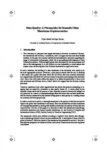
Fig. 2. Best-case interferogram with a centralized centerburst. The y axis is truncated to illustrate the interferogram’s small-scale structure. Inset, region about the centerburst.

calibration procedures, most of these problems result in calibrated spectra that have significant radiance errors. However, in many cases, the interferograms can be processed to yield corrected uncalibrated spectra that then yield accurate calibrated spectra. A.

Fig. 1. Clear-sky spectrum in band 3 of the IMG instrument taken on 24 April 1997 over the Arctic Ocean (80 N, 94 E). (a) Upwelling radiance at the top of the atmosphere. The three black dashed curves are Planck radiance spectra at 240 K, 250 K, and 260 K. (b) Corresponding brightness temperature spectrum with the predominant emission bands labeled.

3. Quality of the Interferometric Monitor for Greenhouse Gases Interferograms

As a first check of the quality of the IMG data, the interferograms are examined. Figure 2 shows a “best-case,” level-0B interferogram, which was obtained during normal operation of the IMG. The inset figure is an expanded view of the region about the interferogram maximum, or centerburst. The interferogram is nearly symmetric about the centerburst. The small asymmetries are related to the fact that the zero path difference (ZPD) of the moving mirror is not sampled exactly, and thus the centerburst is slightly shifted from the ZPD. Also, the point closest to the ZPD may have been removed during data compression. Approximately 31% of all the interferograms are “best-case” data, such as the one shown in Fig. 2. The remaining 69% of interferograms have been identified to have one or more of three types of abnormal features. Once transformed to spectral space, these features introduce abnormalities into the uncalibrated spectra, which then propagate into both the real and imaginary parts of the calibrated spectra. If processed using typical interferometric 522


Data Screening in Interferogram Space

The problematic interferograms exhibit one of the following features: (1) a decentralized centerburst, (2) an extremely asymmetric centerburst region, or (3) noise bursts. Figure 3 displays examples of each of these types of interferograms. Interferograms with decentralized centerbursts could be caused by failure in synchronization of the interferometer mirror movement and data sampling, resulting in improper data acquisition. In normal operation of the instrument, the centerburst will be nearly centered within the interferogram. In practice, it is easy to determine if a decentralized centerburst exists by comparing the center of the interferogram to the location of the centerburst. In this study, a centerburst is classified as decentralized if it is not within 10% of the center of the interferogram. It is difficult to ascertain what causes an extremely asymmetric centerburst region, but it could be improper data acquisition or problems with the travel of the moving mirror near the ZPD. These types of interferograms are difficult to detect in practice because normal interferograms are slightly asymmetric. However, as shown in Fig. 3(b), the asymmetry is sometimes quite noticeable. It was determined that, when present, extreme asymmetries typically occur at the same mirror displacement shown in Fig. 3(b). Therefore, asymmetry is detected by comparing the interferometric values on either side of the centerburst out to the mirror displacement shown in Fig. 3(b), and then determining if they are equal to within a 10% tolerance. Noise bursts in the interferograms might be caused by electromagnetic interference within the IMG

values) and to the right (positive values). For example, the bin labeled −1 contains information about noise bursts located between 10,000 and 20,000 interferogram points to the left of the centerburst; þ3 contains information between 30,000 and 40,000 points to the right of the centerburst. Note that noise bursts near the centerburst (bins −0 and þ0) are undetectable relative to the large signal around the ZPD. The figure shows that the likelihood of noise bursts is not random, but is strongly correlated with the displacement of the moving mirror. For most bins, noise bursts occur less frequently for views of calibration sources than for Earth views, except in bin þ1, where the opposite is true; in this bin, noise bursts occur about 10 times as often in views of the calibration sources as in views of Earth. Overall, noise bursts occur more often on the right-hand side of the ZPD. Table 1 shows the frequency of occurrence of the various types of errors in the interferograms. Noise bursts are quite common, occurring in almost 67% of the data. Thus, a procedure that can correct noise bursts has the potential to improve a significant portion of IMG data. In some cases, the same procedure can be applied to interferograms with decentralized ZPDs. A correction for extremely asymmetric ZPD regions would require a different method; these cases are rare (5.5% of the data), so they are not considered here. B. Correction Procedure for Noise Bursts in Interferograms

For IMG interferograms that are affected by noise bursts, a method is proposed that uses single-sided Fig. 3. Interferograms with (a) a highly decentralized centerburst located near the maximum amplitude, (b) an asymmetric centerburst region (the asymmetry is apparent when amplitudes at about six points on either side of the centerburst are compared), and (c) a large noise burst just to the left of the centerburst (note that the vertical scale is reduced to show the noise burst, and, therefore, the maximum and minimum values of the centerburst are off the scale).

instrument or perhaps interference from other instrumentation aboard the ADEOS spacecraft. Noise bursts can be difficult to detect in an interferogram because the variation of the signal as a function of the mirror path difference in a normal interferogram is large. However, in a normal interferogram, the standard deviation of the signal on one side of the centerburst should be comparable to that on the other side of the centerburst. Therefore, noise bursts are detected by comparing the standard deviations on either side of the centerburst in bins of 10,000 points. If the standard deviations differ by more than a tolerance factor of 3, a noise burst is assumed. Figure 4 shows the frequency of occurrence of noise bursts in the IMG interferograms. Each 10,000-point bin (“Interferometric Bin” in Fig. 4) is expressed as the distance from the centerburst to the left (negative

Fig. 4. Frequency of occurrence and location of noise bursts within IMG interferograms. The x axis designates the distance from the ZPD, in units of 10,000 data points, that the noise burst was found. Negative distances represent points to the left of the ZPD, and positive distances are to the right. 20 January 2010 / Vol. 49, No. 3 / APPLIED OPTICS

523

Table 1.

Occurrence of Abnormal Interferograms

Type of Error

Number

Frequency (%)a

None Noise bursts Decentralized ZPD Asymmetric ZPD

57,303 123,397 489 10,066

31.0 66.9 0.3 5.5

a An interferogram can have more than one type of error; thus, the frequency column totals more than 100%.

interferograms to transform the data to uncalibrated spectra. Single-sided interferograms are constructed using half of the double-sided interferogram, along with a small segment of the other half, close to the ZPD [15]. This can be done as long as the noise burst does not affect data close to the ZPD. A sufficient number of points on the opposite side of the centerburst are needed to properly resolve the phase of the spectrum. Figure 5(a) shows a double-sided interferogram with a noise burst, while Fig. 5(b) shows the corresponding single-sided interferogram. A triangular Mertz apodization function is applied [15] before converting the interferograms to uncalibrated spectra. The single-sided processing makes the interferogram asymmetric, which affects the instrument line shape. In studies that make use of the high spectral resolution, or where matching the instrument line shape is important, an asymmetric apodization function should also be applied to simulated spectra. When single-sided processing is used, we recommend that the asymmetric apodization function be stored with the calibrated radiances, so that it is available for subsequent uses of the data. The Fourier transform of the single-sided interferogram (uncalibrated radiance) is shown in Fig. 6, along with the difference in uncalibrated radiance between the original, double-sided interferogram and the corrected, single-sided interferogram. Note that the effects of the noise bursts in this particular interferogram are clearly visible in the difference curve as both errors over narrow spectral regions (as seen near 860 and 1150 cm−1 ). The differences over broad spectral regions (700–775 cm−1 and 1000– 1075 cm−1 ) are due to differences in the instrumental lineshapes caused by double versus single-sided processing; the errors are the largest where the spectrum is rapidly changing. The largest errors in this uncalibrated radiance spectrum are about 10%–15% and can usually be identified by visual inspection of the uncorrected spectra (not shown). The spectrum created from the single-sided interferogram does not exhibit the errors over the narrow spectral regions, indicating that the single-sided processing effectively corrects for the noise bursts seen in interferogram space. Note that using singlesided interferograms increases the instrument noise in an ideal interferometer by up to a factor of the square root of 2. 524


Fig. 5. (a) Double-sided interferogram measured by the IMG on 2 April 1997 over the Atlantic Ocean (17 S, 33 W). Noise bursts are evident to the right of the ZPD, which is located at an interferogram point number of around 60,000. (b) Corresponding singlesided interferogram with the right portion of the interferogram removed.

4. Quality of the Interferometric Monitor for Greenhouse Gases Spectra A. Calibration of the Interferometric Monitor for Greenhouse Gases Data

The radiometric calibration of interferometric data is described in general terms elsewhere [16]. The calibration procedure for the High-resolution Interferometer Sounder instrument is directly applicable to IMG, since both instruments are Fouriertransform interferometers that use reduction factors to compress data. The basic calibration equation is L ¼ Re½ðCe − Cc Þ=ðCw − Cc Þ&' ðBw − Bc Þ þ Bc ;

ð1Þ

where L is the desired calibrated radiance spectrum, Bw and Bc are the Planck radiances from the warm and cold sources (Bc is effectively zero at infrared wavelengths for IMG calibration), and Ce , Cc , and Cw are uncalibrated spectra of the Earth, space (cold), and warm calibration source, resulting from the Fourier transforms of the interferograms. All variables in Eq. (1) are functions of wavelength. Because the

Fig. 6. (a) Uncalibrated spectrum resulting from taking the Fourier transform of the single-sided interferogram shown in Fig. 5(b) [2 April 1997, (17 S, 33 W)]. (b) Difference in the uncalibrated radiance obtained by subtracting the spectrum obtained with the single-sided interferogram from that using the double-sided interferograms (with noise bursts).

interferograms are asymmetric, whether double- or single-sided, the uncalibrated spectra are complex. Re in Eq. (1) represents the real part of the ratio of the difference spectra inside the square brackets. Since Bw and Bc are real quantities, L is also real. All of the problems with the IMG data that are discussed here can cause asymmetries in the interferograms. These asymmetries are manifested as “signal” in the imaginary part of the calibrated radiance, Limag . If all of the problems are properly addressed, Limag is zero within the instrument noise of IMG. Therefore, the ultimate test of any correction procedure presented here is its ability to yield a calibrated radiance spectrum where Limag is comparable to the noise characteristics of the IMG instrument. B. Resolution of Phase Ambiguities Between Uncalibrated Spectra

Revercomb et al. [16] show that the uncalibrated spectra, C, include both an additive term, due to background radiation from the instrument itself, and a multiplicative term, due to the instrument response. These are removed, respectively, by subtracting the spectra [in the numerator and denominator of Eq. (1)], and taking the ratio of the difference spectra. Taking the ratio also removes the phase response of the instrument. For proper calibration, one must first account for ambiguity in the phases of the uncalibrated radiances: Ce , Cc , and Cw . The phase ambiguity results from the relative distances of the interferogram centerbursts from the true ZPD between views of Earth, space, and the warm calibration source. One method for correcting the anomalous phases of the Tropospheric Infrared Interferometric Sounder, an airborne version of the IMG [13], proposes an iterative method using the

central portion of the interferogram. Here we present a procedure that uses the spectral domain to correct the phases of the individual measurements within a data unit, which gives a unique solution and is noniterative. The shift theorem of Fourier transforms states that a shift in the spatial domain of a series is accom! panied by a corresponding phase shift in the spectral domain: ½f ðX − ΔX ⇔ expði2πΔXνÞf ðνÞ& [17]; the “series” in this case is an interferogram. This change in phase is related to the amount of the relative shift in the interferogram, ΔX, from some reference location, X. Since the sampling of the IMG interferograms is triggered by the helium–neon laser, ΔX is related to the laser wavenumber by ΔX ¼ k=νL, where k is the integral number of points shifted from the reference location. For analysis of the IMG data, the phase of the warm source, ϕw , is used as a reference. The phase ambiguities of the Earth and cold-source measurements are, therefore, determined as the difference in phase from that of the warm source. Here we derive these ambiguities as integer values of k, specific to each measurement. First, the difference in phase of the Earth and cold-source view measurements (ϕx ) within a data unit is determined relative to ϕw as ϕx − ϕw ¼ 2πΔXν ¼ kx ð2πν=νL Þ;

ð2Þ

where x denotes either Earth (e) or cold-source (c) views. Second, the phase ambiguity values, ke ðνÞ and kc ðνÞ, are determined as a function of frequency for each of the Earth and cold-source views as ke ðνÞ ¼ ðϕe − ϕw Þ=ð2πν=νL Þ;

kc ðνÞ ¼ ϕc þ π − ϕw =ð2πν=νL Þ:

ð3Þ

The phase of the cold-source (deep-space) view differs by −π from the other phases because more radiation is emitted from the detector port of the interferometer than from the input port; therefore, the uncalibrated cold-source spectrum must first be multiplied by expðþiπÞ, which is equivalent to adding π to the phase spectrum. Finally, to determine the integral value of k for each measurement, a spectral region must be chosen that does not contain phase anomalies [16]. For IMG band 3, the spectral region from 1200 to 1300 cm−1 is used. ke ðνÞ and kc ðνÞ are averaged over this spectral region, and then the resulting real value is converted to the nearest integer: ! ke ¼ integer½ke ðνÞ&;

! kc ¼ integer½kc ðνÞ&:

ð4Þ

In practice, ke ðvÞ is fairly constant and nearly equal to an integer; however, the values of kc ðvÞ are sometimes more difficult to ascertain. In fact, the departure of kc from an integral value (or ke ) can add a 20 January 2010 / Vol. 49, No. 3 / APPLIED OPTICS

525

small-scale spectral structure to the imaginary part of the calibrated radiance. Once the value of k is known for each measurement within a data unit, the phase ambiguities are eliminated between measurements by either multiplying the original complex, uncalibrated spectrum by expði2πkν=νL Þ or adding 2πkðν=νL Þ to the phase spectrum. Figure 7 shows the phases of uncalibrated IMG spectra before and after the phase ambiguities have been resolved for the measurements made on 2 April 1997. Proper phase resolution is apparent when the phase of the difference spectra in Eq. (1) shows little or no spectral structure. The values of k for the individual measurements in Fig. 7 are þ6, þ7, and 0 for the first Earth view, the coldsource view, and the warm-source view, respectively. For band 3 of the IMG data, k would be 0, (1, or (2 if the phase differences were merely due to the compression of the interferograms, since for band 3 only every third data point is retained. In this case (Fig. 7), the absolute value of k is greater than 2 for the sky

Fig. 7. Phases of individual, uncalibrated radiances from the single-sided interferograms measured on 2 April 1997 [the sky view is from Fig. 6(a)]: (a) before resolving the phase ambiguities and (b) after resolving the phase ambiguities relative to the phase of the warm calibration-source measurement. The lower phase spectrum in (b) is that of the cold calibration view of space, which differs from the other views by approximately −π at wavenumbers larger than about 1100 cm−1 . 526


and cold-source views, so the location of the centerburst must have changed by more than the reduction factor from one measurement to the next, indicating that the ZPD location is shifting between measurements within a data unit. Figure 8 shows the calibrated radiance spectrum for the same data shown in Fig. 7 (2 April 1997): (a) shows the real and imaginary parts of the calibrated spectrum before resolution of phase ambiguities, while (b) shows them after resolution. Before resolving the phase ambiguities, the spectrum is unusable since the real part is actually negative and the imaginary part is quite large and positive. After phase resolution, the real part is positive, and the imaginary part is small and nearly equal to the noise equivalent spectral radiance (NESR) of the IMG’s band 3. [Fig. 3 of Amato et al. [3] shows that the NESR for this band ranges from about 0.3 to 0:6 mW m−2 sr−1 ðcm−1 Þ−1 ]. These NESR values were confirmed here by taking the standard deviation of the detrended calibrated radiance in several microwindows between strong absorption lines.] There is a small amount of residual spectral structure in the imaginary part of the calibrated radiance that

Fig. 8. Calibrated radiance spectra for measurements shown in Fig. 7 [2 April 1997; (17 S, 33 W)]: (a) before and (b) after resolving phase ambiguities. Phase ambiguities can result in significant imaginary parts of calibrated spectra [upper curve in (a)], which are removed by resolving phase ambiguities [lower curve in (b)].

is related to the nonintegral value of kc ðvÞ, as described above, but the resulting Limag is typically less than twice the NESR at most wavenumbers. Any spectral structure in Limag effectively biases the real part of the calibrated radiance. (Limag can actually be minimized further by relaxing the requirement that kc and ke must be integers; this is equivalent to assuming that the ZPD is not stationary within an IMG data unit, which seems plausible.) If either ke or kc is miscalculated by even (1, Limag is greatly increased, making this a sensitive test as to whether or not the phase ambiguities have been properly resolved. Previous works [18] have used various techniques using spectral thresholds to provide quality control on IMG spectra and to categorize the data (e.g., clear versus cloudy). We recommend, instead, that the correction method described here be applied to IMG spectra and that the quality control on these spectra be accomplished by comparing the imaginary part of the calibrated radiance, Limag , to the instrument noise. It is important to note that IMG spectra may look quite reasonable upon visual inspection, yet still have unresolved phase ambiguities. Therefore, certain spectra may appear to be properly calibrated, when in fact they are not. Figure 9 shows the radi-

ance and brightness temperature spectra before and after resolving the phase ambiguities for an IMG measurement made over Indonesia on 15 October 1996. (The value of k for the sky view is þ1 for this case.) The spectra are similar in terms of spectral features, although the radiances and corresponding brightness temperatures after resolving the phase ambiguities are higher (by as much as 10 K in brightness temperature) than those before the correction. Given the latitude of this particular scene (1.3 S, 113.4 E), this measurement is most likely that of a high cloud. The brightness temperatures in the transparent window region between 800 and 1200 cm−1 are about 260–265 K after phase resolution and 250–255 K before phase resolution. If cloud properties are retrieved using the spectrum before phase ambiguities are resolved, errors will result both because of the difference in radiance (brightness temperature) and the slight spectral feature seen around 850 cm−1 . A spectral distortion was previously identified in IMG spectra and correctly attributed to phase mismatching [18]. Since a correction procedure did not exist at that time, spectra had to be screened out manually, which proved “tedious and long.” If not correctly identified and screened out, these errors would be detrimental to those using IMG data for studies that require a high degree of radiometric accuracy, such as the retrieval of atmospheric properties. 5.

Fig. 9. (a) Calibration radiance and (b) brightness temperature spectra for an IMG measurement made over Indonesia (1.3 S, 113.4 E) on 15 October 1996. Spectra are shown both before and after resolving phase ambiguities in the uncalibrated spectra.

Conclusions

We have identified errors in IMG interferograms due to noise bursts, extreme asymmetries about the centerburst, decentralized centerbursts, and unresolved phase ambiguities. The errors due to noise bursts can be avoided for many interferograms by constructing a single-sided interferogram from the original, double-sided interferograms. Single-sided interferograms include half of the interferogram on one side of the ZPD, as well as a short section on the other side near the ZPD. The number of points to include in the short section depends on the number of error-free points about the centerburst; using fewer points will introduce higher noise into the calibrated radiance (an increase of up to the square root of 2) and result in a lower-resolution phase spectrum. Since an apodization function must be applied in the single-sided processing of interferograms, the same apodization function should be applied to simulated spectra to match the instrument line shape. In this work, the correction procedure is applied to noise bursts, which represent the vast majority of the errors. However, this procedure could also be applied to interferograms with a decentralized ZPD. Before radiometric calibration, it is essential to resolve any phase ambiguities in the interferograms caused by shifts in the positions of the ZPD between interferograms of Earth and space views relative to the warm calibration-source view. These ambiguities occur in the IMG data because of data compression and perhaps improper tracking of the interferometer’s 20 January 2010 / Vol. 49, No. 3 / APPLIED OPTICS

527

scan mirror. If phase ambiguities are present but not corrected for, large errors in the spectrum will result. These errors may cause a distortion in the spectral shape that is obvious upon visual inspection, but they may also cause a fairly smooth bias that might remain unnoticed despite biases as large as 10 K in brightness temperature. A method for correcting for phase ambiguities in the spectral domain is presented. These quality-control procedures are essential to ensure high-quality radiance spectra from the IMG instrument for a range of important studies of the Earth’s atmosphere, including determining longterm trends in atmospheric variables. We gratefully acknowledge the receipt of IMG data from the Earth Remote Sensing Data Analysis Center in Japan and, specifically, Ryoichi Imasu and Hidemichi Saji for their help. We had useful discussions about the calibration and interpretation of IMG data with Kayoko Kondo (Toshiba Corporation). We also acknowledge the helpful comments of two anonymous reviewers. Early progress on this project was funded by the International Arctic Research Center, University of Alaska Fairbanks and the National Aeronautics and Space Administration (NASA) Headquarters through Ramesh Kakar. Funding was also supplied by the National Aeronautics and Space Administration (NASA) Research Opportunities in Space and Earth Sciences program (Contract NNX08AF79G). References 1. H. Kobayashi, A. Shimota, K. Kondo, E. Okumura, Y. Kameda, H. Shimoda, and T. Ogawa, “Development and evaluation of the interferometric monitor for greenhouse gases: a highthroughput Fourier-transform infrared radiometer for nadir Earth observation,” Appl. Opt. 38, 6801–6807 (1999). 2. J. Wang, J. C. Gille, H. E. Revercomb, and V. P. Walden, “Validation study of the MOPITT retrieval algorithm: carbon monoxide retrieval from IMG observations during WINCE,” J. Atmos. Ocean. Technol. 17, 1285–1295 (2000). 3. U. Amato, V. Cuomo, I. De Feis, F. Romano, C. Serio, and H. Kobayashi, “Inverting for geophysical parameters from IMG radiances,” IEEE Trans. Geosci. Remote Sensing 37, 1620–1632 (1999). 4. A. M. Lubrano, C. Serio, S. A. Clough, and H. Kobayashi, “Simultaneous inversion for temperature and water vapor from IMG radiances,” Geophys. Res. Lett. 27, 2533–2536 (2000). 5. C. Clerbaux, J. Hadji-Lazaro, S. Turquety, G. Mégie, and P.-F. Coheur, “Trace gas measurements from infrared satellite

528


6.

7.

8.

9.

10.

11.

12.

13.

14.

15. 16.

17. 18.

for chemistry and climate applications,” Atmos. Chem. Phys. 3, 1495–1508 (2003). R. A. Hanel, B. Schlachman, D. Rogers, and D. Vanous, “Nimbus 4 Michelson interferometer,” Appl. Opt. 10, 1376– 1382 (1971). J. E. Harries, H. E. Brindley, P. J. Sagoo, and R. J. Bantges, “Increases in greenhouse forcing inferred from the outgoing longwave radiation spectra of the Earth in 1970 and 1997,” Nature 410, 355–357 (2001). H. H. Aumann, M. T. Chahine, C. Gautier, M. D. Goldberg, E. Kalnay, L. M. McMillin, H. Revercomb, P. W. Rosenkranz, W. L. Smith, D. H. Staelin, L. L. Strow, and J. Susskind, “AIRS/ AMSU/HSB on the Aqua mission: design, science objectives, data products, and processing systems,” IEEE Trans. Geosci. Remote Sensing 41, 253–264 (2003). A. B. Uspensky, I. V. Cherny, G. M. Chernyavsky, Y. M. Golovin, F. S. Zavelevich, A. K. Gorodetsky, B. E. Moshkin, G. G. Gorbunov, and A. S. Romanovsky, “Sounding instruments for future Russian meteorological satellites,” Technical Proceedings of the 10th International TOVS Study Conference (1999), pp. 533–543. Available from the co-chairs of the International TOVS Working Group, http://cimss.ssec.wisc .edu/itwg. D. Blumstein, B. Tournier, F. R. Cayla, T. Phulpin, R. Fjortoft, C. Buil, and G. Ponce, “In-flight performance of the Infrared Atmospheric Sounding Interferometer (IASI) on METOP-A,” Proc. SPIE 6684, 66840H (2007). National Institute for Environmental Studies (NIES) Greenhouse Gases Observing Satellite (GOSAT) Project, GOSAT pamphlet (Center for Global Environmental Research and National Institute for Environmental Studies, 2006). H. J. Bloom, “The Cross-track Infrared Sounder (CrIS): a sensor for operational meteorological remote sensing,” in Geoscience and Remote Sensing Symposium (IGARSS International, 2001), Vol. 3, pp. 1341–1343. A. Shimota, H. Kobayashi, and S. Kadokura, “Radiometric calibration for the airborne interferometric monitor for greenhouse gases simulator,” Appl. Opt. 38, 571–576 (1999). H. Kobayashi, ed., “Interferometric monitor for greenhouse gases,” Tech. Rep. (Interferometric Monitor for Greenhouse Gases Project, 1999), p. 45. P. R. Grifﬁths and J. A. deHaseth, Fourier Transform Infrared Spectrometry (Wiley, 1986). H. E. Revercomb, H. Buijs, H. B. Howell, D. D. LaPorte, W. L. Smith, and L. A. Sromovsky, “Radiometric calibration of IR Fourier transform spectrometers: solution to a problem with the High-Resolution Interferometer Sounder,” Appl. Opt. 27, 3210–3218 (1988). R. N. Bracewell, The Fourier Transform and Its Applications, 2nd ed. (McGraw-Hill, 1986), p. 474. G. Masiello, C. Serio, and H. Shimoda, “Qualifying IMG tropical spectra for clear sky,” J. Quant. Spectr. Rad. Trans. 77, 131–148 (2003).