Improving Classification Accuracy of Large Test ... - Semantic Scholar
Recommend Documents
26 multimodal MRI-WMH image pairs, all four registration methods produced a higher area under the receiver operating characteristic curve compared to that obtained from expert ... Despite possession of empirical domain knowledge by the.
multi-VDD conditions: application to envelope-based test of LNAs. Manuel J. ... on ensemble learning of digital envelope signatures [5]. This paper is organized ...
Oct 26, 2011 - classifying normal heartbeats, Premature Ventricular Contraction. (PVC) and ... recordings contain complex ventricular, junctional and supra.
Justin Fackrell, Wojciech Skut and Kathrine Hammervold. Rhetorical Systems Ltd. 4 Crichton's Close, Canongate,. Edinburgh, UK [email protected].
In recent research, multivariate analysis of Positron Emission. Tomography (PET) datasets ... Health Science Centre, Wolfson Molecular Imaging Centre, The University of Manchester, Manchester ... URN: http://nbn-resolving.de/urn:nbn:de:bsz:352-opus-9
It is also the state-of-the-art on Chi- nese SRC. 1 Introduction. Semantic Role labeling (SRL) was first defined in. Gildea and Jurafsky (2002). The purpose of SRL.
May 21, 2014 - Article. Improving Classification of Airborne Laser Scanning Echoes in the Forest-Tundra Ecotone Using Geostatistical and Statistical Measures.
Jul 24, 2015 - ... AZ, USA, 3 Department of. Computational Medicine and Bioinformatics, University of Michigan, Ann Arbor, MI, USA, 4 Department of Electrical ..... mini-mental state exam (MMSE) and the clinical dementia rating (CDR) are ...... http:
1805 N. Broad Street,. Philadelphia, PA 19122. USA. {qfxu, zoran, hanbo, liyong, [email protected]}. 2California Institute of Technology,. 4800 Oak Grove ...
enhance consumer experiences (Gaukler and Hausman, 2008;. Johansson and Hellström, 2007; Kärkkäinen, 2003; Wong and. McFarlane, 2007). Furthermore ...
enhance accuracy of the available bandwidth estimation in IEEE ... combines medium state monitoring, probability of collision .... free. As this method is solely based on a signal level measurement, it allows taking into account emissions.
important issue in data mining. ... Removing the noise and outliers during training allows the learning .... the filtered dataset for training and the whole data set for.
ensemble model is proposed to improve classification accuracy. Feature selection ..... QUEST is a binary classification method [6] for building decision trees.
Email: [email protected] ... NFCV-driven automated parameter selection yielded a classification accuracy of 82.94% compared to ... Common BCI application platforms are cursor control (Trejo et al., 2006), spelling systems ...
curacy gains using automatically extracted training data at much lower cost. Categories ... task of inferring whether a query posed to a search engine has commercial intent ...... Optimizing search engines using clickthrough data. In KDD, pages ...
sectors, providing a link from company names to sector labels in the ..... example, if company X is described in the text as âsoftware companyâ we can assume.
single classifier [2,6,7,3], as opposed to multi-classifier and multimodal ... two different face image matchers, a quality measure that is correlated with the.
We evaluated classification performance with Relative Classifier. Information (RCI). RCI is an entropy-based performance measure that quantifies the amount of.
Sep 8, 2016 - Lateral l. Stop. b p d t g h. Fricative. z c zh ch j q. Retroflex zh ch sh r. Alveolar ... place voiced nasal /n/ with lateral /l/ and back nasals with their.
Microsoft internal large vocabulary telephony speech recognition task (with 2000 hours of training ..... MSCT 70K. 4356. General call center application. STK 40K.
Jul 27, 2016 - ner (Signa VHi; General Electric Healthcare, Waukesha, WI, USA) equipped with an eight-channel, phased-array head coil. For each par-.
being applied onto a distributed application namely Coronary Disease data set ... being applied on a single standalone application leading to the emergence of ..... [20] Antunes SG, Silva JS, Santos JB, Martins P, Castela E, âPhase Symmetry.
tral frequencies (LSF), the energy and its delta and the zero crossing rate of ... zero magnitude and the number of signal samples existing in a fixed size window.
Improving Classification Accuracy of Large Test ... - Semantic Scholar
We present a new algorithm called Ordered Classification, that is useful ... nomical task of automated prediction of stellar atmospheric parameters, as well as to ...
Improving Classification Accuracy of Large Test Sets Using the Ordered Classification Algorithm Thamar Solorio1 and Olac Fuentes1 ´ Instituto Nacional de Astrof´ısica, Optica y Electr´ onica, Luis Enrique Erro # 1, 72840 Puebla, M´exico [email protected], [email protected]
Abstract. We present a new algorithm called Ordered Classification, that is useful for classification problems where only few labeled examples are available but a large test set needs to be classified. In many real-world classification problems, it is expensive and some times unfeasible to acquire a large training set, thus, traditional supervised learning algorithms often perform poorly. In our algorithm, classification is performed by a discriminant approach similar to that of Query By Committee within the active learning setting. The method was applied to the real-world astronomical task of automated prediction of stellar atmospheric parameters, as well as to some benchmark learning problems showing a considerable improvement in classification accuracy over conventional algorithms.
1
Introduction
Standard supervised learning algorithms such as decision trees (e.g. [1, 2]), instance based learning (e.g. [3]), Bayesian learning and neural networks require a large training set in order to obtain a good approximation of the concept to be learned. This training set consists of instances or examples that have been manually, or semi-manually, analyzed and classified by human experts. The cost and time of having human experts performing this task is what makes unfeasible the job of building automated classifiers with traditional approaches in some domains. In many real-world classification problems we do not have a large enough collection of labeled samples to build an accurate classifier. The purpose of our work is to develop new methods for reducing the number of examples needed for training by taking advantage of large test sets. Given that the problem setting described above is very common, an increasing interest from the machine learning community has arisen with the aim of designing new methods that take advantage of unlabeled data. By allowing the learners to effectively use the large amounts of unlabeled data available, the size of the manual labeled training sets can be reduced. Hence, the cost and time needed for building good classifiers will be reduced, too. Among the most popular methods proposed for incorporating unlabeled data are the ones based on a generative model, such as Naive Bayes algorithm in combination with the Expectation Maximization (EM) algorithm [4–8]. While this approach has proven
to increase classifier accuracy in some problem domains, it is not always applicable since violations to the assumptions made by the Naive Bayes classifier will deteriorate the final classifier performance [9, 10]. A different approach is that of co-training [11, 10], where the attributes describing the instances can naturally be divided into two disjoint sets, each being sufficient for perfect classification. One drawback of this co-training method is that not all classification problems have instances with two redundant views. This difficulty may be overcome with the co-training method proposed by Goldman and Zhou [12], where two different learning algorithms are used for bootstrapping from unlabeled data. Other proposals for the use of unlabeled data include the use of neural networks [13], graph mincuts [14], Semi-Supervised Support Vector Machines [15] and Kernel Expansions [16], among others. In this paper we address the problem of building accurate classifiers when the labeled data are insufficient but a large test set is available. We propose a method called Ordered Classification (OC), where all the unlabeled data available are considered as part of the test set. Classification with the OC is performed by a discriminant approach similar to that of Query By Committee within the active learning setting [17–19]. In the OC setting, the test set is presented to an ensemble of classifiers built using the labeled examples. The ensemble assigns labels to the entire test set and measures the degree of confidence in its predictions for each example in the test set. According to a selection criterion examples with a high confidence level are chosen from the test set and used for building a new ensemble of classifiers. This process is repeated until all the examples from the test set are classified. We present some experimental results of applying the OC to some benchmark problems taken from the UCI Machine Learning Repository [20]. Also, as we are interested in the performance of this algorithm in real-world problems, we evaluate it on a data set obtained from a star catalog due to Jones [21] where the learning problem consists in predicting the atmospheric parameters of stars from spectral indices. Both types of experiments show that using the OC results in a considerable decrease of the prediction error.
2
The Ordered Classification Algorithm
The goal of the OC algorithm is to select those examples whose class can be predicted by the ensemble with a high confidence level in order to use them to improve its learning process by gradually augmenting an originally small training set. How can we measure this confidence level? Inspired by the selection criterion used in previous works within the active learning setting (e.g. [17– 19]) we measure the degree of agreement among the members of the ensemble. For real-valued target functions, the confidence level is given by the inverse of the standard deviation on the predictions of the ensemble. Examples with low standard deviation in their predicted target function are considered more likely to be correctly classified by the ensemble, thus these examples are selected and added to the training set. For discrete target functions we measure the confidence
level by computing the entropy on the classifications made by the ensemble on the test set. Again, examples with low entropy values are selected for rebuilding the ensemble. The test set is considered as the unlabeled data since they do not have a label indicating their class, so from now on we will use the words unlabeled data and test set to refer to the same set. Our algorithm proceeds as follows: First, we build several classifiers (the ensemble) using the base learning algorithm and the training set available. Then, each classifier predicts the classes for the unlabeled data and we use these predictions to estimate the reliability of the predictions for each example. We now proceed to select the n previously unlabeled examples with the highest confidence level and add them to the training set. Also, the ensemble re-classifies all the examples added until then, if the confidence level is higher than the previous value then the labels of the examples are changed. This process is repeated until there are no unlabeled examples left. See Table 1 for an outline of our algorithm. The OC can be used in combination with any supervised learning algorithm. In the experimental results presented here, when the learning task involves realvalued target functions we used Locally Weighted Linear Regression (LWLR) [3]; for discrete-valued target functions we used C4.5 [2]. The next subsections briefly describe these learning algorithms. 2.1
Ensembles
An ensemble of classifiers is a set of classifiers whose individual decisions are combined in some way, normally by voting. In order for an ensemble to work properly, individual members of the ensemble need to have uncorrelated errors and an accuracy higher than random guessing. There are several methods for building ensembles. One of them, which is called bagging [22], consists of manipulating the training set. In this technique, each member of the ensemble has a training set consisting of m examples selected randomly with replacement from the original training set of m examples (Dietterich [23]). Another technique similar to bagging manipulates the attribute set. Here, each member of the ensemble uses a different subset randomly chosen from the attribute set. More information concerning ensemble methods, such as boosting and error-correcting output coding, can be found in [23]. The technique used for building an ensemble is chosen according to the learning algorithm used, which in turn is determined by the learning task. In the work presented here, we use bagging when C4.5 [2] is the base learning algorithm; and the one that randomly selects attributes when using Locally Weighted Regression [3]. 2.2
The Base Learning Algorithm C4.5
C4.5 is an extension to the decision-tree learning algorithm ID3 [1]. Only a brief description of the method is given here, more information can be found in [2]. The algorithm consists of the following steps: 1. Build the decision tree form the training set (conventional ID3).
Table 1. The ordered classification algorithm Is is a matrix whose rows are vectors of attribute values Ls is the class label S is the training set, given by the tuple [Is , Ls ] U is the unlabeled test set A is initially empty and will contain the unlabeled examples added to the training set 1. While U 6= do: – Construct E, the ensemble containing k classifiers – Classify U and estimate reliability of predictions – V are the n elements of U for which the classification assigned by the ensemble is most reliable – S =S∪V – U =U −V – A=A∪V – Classify A using E and change the labels of the examples with higher confidence level 2. End
2. Convert the resulting tree into an equivalent set of rules. The number of rules is equivalent to the number of possible paths from the root to a leaf node. 3. Prune each rule by removing any preconditions that result in improving its accuracy, according to a validation set. 4. Sort the pruned rules in descending order according to their accuracy, and consider them in this sequence when classifying subsequent instances. Since the learning tasks used to evaluate this work involve nominal and numeric values, we implemented the version of C4.5 that incorporates continuous values. 2.3
Locally Weighted Linear Regression
LWLR belongs to the family of instance-based learning algorithms. These algorithms build query specific local models, which attempt to fit the training examples only in a region around the query point. They simply store some or all of the training examples and postpone any generalization until a new instance must be classified. In this work we used a linear model around the query point to approximate the target function. Given a query point xq , to predict its output parameters yq , we assign to each example in the training set a weight given by the inverse of the distance 1 from the training point to the query point: wi = |xq −x i| Let W , the weight matrix, be a diagonal matrix with entries w1 , . . . , wn . Let X be a matrix whose rows are the vectors x1 , . . . , xn , the input parameters of the examples in the training set, with the addition of a “1” in the last column. Let Y be a matrix whose rows are the vectors y1 , . . . , yn , the output parameters
of the examples in the training set. Then the weighted training data are given by Z = W X and the weighted target function is V = W Y . Then we use the estimator for the target function yq = xTq (Z T Z)−1 Z T V. Table 2. Description of Data sets name chess lymphography credit soybean spectral indices
In order to assess the effectiveness of the OC algorithm we experimented on some learning tasks taken from the UCI Machine Learning Repository [20] as well as on an astronomical data set of spectral indices due to Jones [21]. In Table 2 we present a description of each data set used. In all the experiments reported here we used the evaluation technique 10-fold cross-validation, which consists of randomly dividing the data into 10 equallysized subgroups and performing ten different experiments. We separated one group along with their original labels as the validation set; another group was considered as the starting training set; the remainder of the data were considered the test set. Each experiment consists of ten runs of the procedure described above, and the overall average are the results reported here. 3.1
Benchmark Experiments
We described in this subsection the experiments with the data sets of the UCI Machine Learning Repository. To analyze the effectiveness of the Ordered Classification algorithm we performed three different experiments and compared the resulting accuracy. In the first type of experiment we built an ensemble of classifiers, with seven members, using C4.5 and the training set available. The test set was then classified by this ensemble and the resulting classification error rates are presented in Table 3 under the column named standard. In the next type of experiment we built again an ensemble with seven members, C4.5 and the training set available. This time a random selection of n examples from the test set was made and added to the training set until the complete test set was classified. | We set n = |T 10 , where T is the training set. The error rates for this experiment are also in Table 3 under the feature random selection. The column named OC presents the results of experimenting using our algorithm. Parameters k and n where set to the same values as the previous experiment.
Table 3. Comparison of the error rates
lymphography chess soybean credita
standard random selection 0.2912 0.2668 0.0551 0.0523 0.2714 0.2255 0.0952 0.0915
OC 0.2567 0.0419 0.1947 0.0848
The main difference between random selection and the OC algorithm is that the former does not measures the confidence level on the predictions of the ensemble, it simply selects randomly which unlabeled examples are going to be added in the training process. We performed the random selection experiment with the purpose of finding if the selection criterion used in the OC algorithm gives better results than simply using labeled examples selected randomly. Unsurprisingly, the error rates of random selection are lower than the traditional C4.5, but in all the learning tasks, the lowest error rates were obtained with our algorithm. We can notice that by incrementally augmenting a small training set we can boost accuracy of standard algorithms. The advantage of using our algorithm over random selection is that we are maximizing the information gained by carefully selecting unlabeled data, and that is the reason why we can improve further classifier accuracy. For these benchmark problems error reductions of up to 29% were attained. Results from Table 3 suggest that the OC algorithm is the best alternative.
−13
4.5
x 10
4
3.5
3
Flux
2.5
2
1.5
1
0.5
0 3800
3900
4000
4100
4200
4300
Wavelength
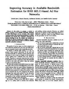
Fig. 1. Stellar spectrum
4400
4500
4600
Table 4. Comparison of mean absolute errors in the prediction of stellar atmospheric parameters
Teff[K] Log g[dex] Fe/H
3.2
traditional random selection 147.33 133.79 0.3221 0.3030 0.223 0.177
OC 126.88 0.2833 0.172
Prediction of Stellar Atmospheric Parameters
We introduce here the problem of automated prediction of stellar atmospheric parameters. As mentioned earlier, we are interested in the applicability of our algorithm to real-world problems. Besides, we know that important contributions might emerge from the collaboration of computer science researchers with researchers from different scientific disciplines. In order to predict some physical properties of a star, astronomers analyze its spectrum, which is a plot of energy flux against wavelength. The spectra of stars consists of a continuum, with discontinuities superimposed, called spectral lines. These spectral lines are mostly dark absorbtion lines, although some objects can present bright emission lines. By studying the strength of various absorption lines, temperature, composition and surface gravity can be deduced. Figure 1 shows the spectrum of a star from the data set we are using. Instead of using the spectra as input data, a very large degree of compression can be attained if we use a measurement of the strength of several selected absorption lines that are known to be important for predicting the stellar atmospheric parameters. In this work we use a library of such measurements, which are called spectral indices in the astronomical literature, due to Jones [21]. This dataset consists of 24 spectral indices for 651 stars, together with their estimated effective temperatures, surface gravities and metallicities. It was observed at Kitt Peak National Observatory and has been made available by the author at an anonymous ftp site at the National Optical Astronomy Observatories(NOAO). For the learning task of predicting stellar atmospheric parameters we used LWLR as the base learning algorithm. Results from the experiments are presented in Table 4, which presents the mean absolute errors for the three types of experiments performed. Each experiment was carried out as explained in the previous subsection. We can observe that the lowest error rates were attained when using our algorithm. An error decrease of up to 14% was reached taking advantage of the large test set available. However, both learners that used unlabeled data outperformed the traditional Locally Weighted Linear Regression Algorithm. A different experiment was performed to analyze the effect of using the OC algorithm with training sets of different sizes. Figure 2 shows a graphical comparison of predicting the stellar atmospheric parameter metallicity using an ensemble of LWLR and the OC algorithm. From these results we can conclude that even when standard LWLR performs satisfactory well with a large enough
training set, OC can take advantage of the test set and outperform accuracy of LWLR. 0.3 Ensemble LWLR The OC algorithm
0.25
Error rate
0.2
0.15
0.1
0.05 0
100
200 300 400 Number of examples used for training
500
600
Fig. 2. Error Comparison between an ensemble of LWLR and the OC algorithm as the number of training examples increases
4
Conclusions
The Ordered Classification algorithm presented here was successfully applied to the problem of automated prediction of stellar atmospheric parameters, as well as evaluated with some benchmark problems proving in both cases to be an excellent alternative when the labeled data are scarce and expensive to obtain. Results presented here prove that poor performance of classifiers due to a small training sets can be improved upon when a large test set is available or can be gathered easily. One important feature of our method is the criterion by which we select the unlabeled examples from the test set -the confidence level estimation. This selection criterion allows the ensemble to add new instances that will help obtain a better approximation of the target function; but at the same time, this discriminative criterion decreases the likelihood of hurting the final classifier performance, a common situation when using unlabeled data. From experimental results we can conclude that unlabeled data selected randomly improve the accuracy of standard algorithms, moreover, a significant further improvement can be attained when we use the selection criterion proposed in this work. Another advantage of the algorithm presented here is that it is easy to implement and given that it can be applied in combination with almost any supervised learning algorithm, the possible application fields are unlimited.
One disadvantage of this algorithm is the computational cost involved. As expected, the running time of our algorithm increases with the size of the test set. It evaluates the reliability of every single examples in the test set, thus the computational cost is higher than traditional machine learning approaches. However, if we consider the time and cost needed for gathering a large enough training set, for traditional algorithms, our approach is still more practical and feasible. Some directions of future work include: – – – –
Extending this methodology to other astronomical applications. Performing experiments with a different measure of the confidence level. Experimenting with a heterogeneous ensemble of classifiers. Performing experiments with other base algorithms such as neural networks.
References 1. J.R. Quinlan. Induction of decision trees. Machine Learning, 1:81–106, 1986. 2. J.R. Quinlan. C4.5: Programs for machine learning. 1993. San Mateo, CA: Morgan Kaufmann. 3. Christopher G. Atkeson, Andrew W. Moore, and Stefan Schaal. Locally weighted learning. Artificial Intelligence Review, 11:11–73, 1997. 4. A. McCallum and K. Nigam. Employing EM in pool-based active learning for text classification. In Proceedings of the 15th International Conference on Machine Learning, 1998. 5. K. Nigam, A. Mc Callum, S. Thrun, and T. Mitchell. Learning to classify text from labeled and unlabeled documents. Machine Learning, pages 1–22, 1999. 6. K. Nigam. Using Unlabeled Data to Improve Text Classification. PhD thesis, Carnegie Mellon University, 2001. 7. S. Baluja. Probabilistic modeling for face orientation discrimination: Learning from labeled and unlabeled data. Neural Information Processing Sys., pages 854–860, 1998. 8. B. Shahshahani and D. Landgrebe. The effect of unlabeled samples in reducing the small sample size problem and mitigating the Hughes phenomenon. IEEE Transactions on Geoscience and Remote Sensing, 32(5):1087–1095, 1994. 9. F. Cozman and I. Cohen. Unlabeled data can degrade classification performance of generative classifiers. Technical Report HPL-2001-234, Hewlett-Packard Laboratories, 1501 Page Mill Road, September 2001. 10. K. Nigam and R. Ghani. Analyzing the effectiveness and applicabitily of cotraining. Ninth International Conference on Information and Knowledgement Management, pages 86–93, 2000. 11. A.Blum and T. Mitchell. Combining labeled and unlabeled data with co-training. In Proceedings of the 1998 Conference on Computational Learning Theory, July 1998. 12. S. Goldman and Y. Zhou. Enhancing supervised learning with unlabeled data. In Proceedings on the Seventeenth International Conference on Machine Learning: ICML-2000, 2000. 13. M.T. Fardanesh and K.E. Okan. Classification accuracy improvement of neural network by using unlabeled data. IEEE Transactions on Geoscience and Remote Sensing, 36(3):1020–1025, 1998.
14. A. Blum and Shuchi Chawla. Learning from labeled and unlabeled data using graph mincuts. ICML’01, pages 19–26, 2001. 15. G. Fung and O.L. Mangasarian. Semi-supervised support vector machines for unlabeled data classification. Optimization Methods and Software, (15):29–44, 2001. 16. M. Szummer and T. Jaakkola. Kernel expansions with unlabeled examples. NIPS 13, 2000. 17. Y. Freund, H. Seung, E. Shamir, and N. Tishby. Selective sampling using the query by comitee algorithm. Machine Learning, 28(2/3):133–168, 1997. 18. S. Argamon-Engelson and I. Dagan. Committee-based sample selection for probabilistic classifiers. Journal of Artificial Inteligence Research, (11):335–360, Nov. 1999. 19. R. Liere and Prasad Tadepalli. Active learning with committees for text categorization. In Proceedings of the Fourteenth National Conference on Artificial Intellignce, pages 591–596, 1997. 20. C. Merz and P. Murphy. UCI Machine Learning Repository. http://www.ics.uci.edu./∼mlearn/MLRepository.html, 1996. 21. L.A. Jones. Star Populations in Galaxies. PhD thesis, University of North Carolina, Chapel Hill, North Carolina, 1996. 22. L. Breiman. Bagging predictors. Machine Learning, 24(2):123–140, 1996. 23. T. Dietterich. Ensemble methods in machine learning. In First International Workshop on Multiple Classifier Systems, Lecture Notes in Computer Science, pages 1–15, New York: Springer Verlag, 2000. In J. Kittler and F. Roli (Ed.).