Mel-frequency cepstral coefficients under both of the two protocols. 1. ..... References. [1] S. B. Davis and P. Mermelstein, âComparison of. Parametric ...
Improving Performance of Text-Independent Speaker Identification by Utilizing Contextual Principal Curves Filtering Yong Guan Hongwei Qi Wenju Liu and Jue Wang National Lab. of Pattern Recognition, Institute of Automation, Chinese Academy of Sciences, Beijing, China, 100080 {yguan,lwj}@nlpr.ia.ac.cn
Abstract In this paper, a novel filtering method in feature extraction of speech is proposed for text-independent speaker identification, called Contextual Principal Curves Filtering (CPCF). The CPCF provides a good nonlinear summary of a sequence of cepstral vectors on the time context and, the most important, keeps their intrinsic trajectory characteristics, so the CPCF algorithm do improve the cepstral coefficients to represent speech feature more precisely. We apply this CPCF algorithm into two protocols in the framework of close-set textindependent speaker identification, where the experimental data are collected from a subset of 863 speech database of China National High Technology Project. The results show a steady relative error rate reduction of the identification for more than 20% compared with the use of the conventional Mel-frequency cepstral coefficients under both of the two protocols.�
1. Introduction It is well-known that the performance of the text-independent speaker identification (TI-SID) can be improved from three aspects: feature extraction, model training and scoringdecision. To hunt the potential high performance of the TISID, finding a more intrinsic speech feature is a more essential way than improving the efficiency of the other two aspects and it is also what this paper aims at. Mel-Frequency Cepstral coefficients (MFCCs) [1] have been widely used in feature extraction of speech processing for speaker recognition as well as speech recognition. Although MFCC, which reflects a person’s vocal tract structure distinguishing the given person from the others, provides a good set of feature vectors with nice properties, we convince that they are not good enough to represent speech signals in most situations, especially in speaker recognition. To find a good improvement to MFCC, a lot of approaches have been introduced in recent years, such as its delta and delta-delta coefficients [2], which are used to capture more dynamic information. In this paper, we evaluate the information of cepstral vectors by variance and present a new filtering method based on principal curves. Since the principal curves algorithm is applied as a filtering method to cepstral vectors and their time contexts (a sequence of cepstral vectors), we call it Contextual Principal Curves Filtering (CPCF) of speech. In this algorithm, the total variance of the cepstral vectors is
This work was supported by National Key Project for Basic Research in China (G1998030508), China National Nature Science Foundation (No.60172055) and Beijing Nature Science Foundation (No.4042025).
decomposed into the intrinsic information explained by the true principal curve and the noise information in the expected squared distance from a point to its projection on the curve. The CPCF algorithm, which extracts the intrinsic information of the cepstral vectors with getting rid of the noise, provides good nonlinear summary of the cepstral vectors on the time contexts and, the most important, keeps their intrinsic trajectory characteristics. We finally apply the CPCF algorithm in the framework of closed-set text-independent speaker identification. We perform the CPCF to filtering a sequence of log-energy vectors before cosine transform as well as directly to filtering a sequence of final cepstral vectors while extracting the speech features. The results show that a considerable more than 20% relative error rate reduction of identification is gained compared with the use of conventional MFCC in the former case under two protocols with different scoring. The outline of this paper is the following. Section 2 introduces the principal curve and presents the Contexture Principal Curves Filtering algorithm used in the experiments. Then how to integrate the CPCF in a speaker identification system is explained in section 3. The organization and the results of the experiments are showed in section 4. Section 5 concludes our study.
2.
The Principal Curves
Principal Curves (henceforth PCs), presented by Hastie and Stuetzle in 1988 [3], represent smooth one-dimensional curves passing through the ‘middle’ of the dataset. From the view of probability distribution, PCs satisfy the self-consistent property. PCs, the natural non-linear generalization of linear principal components, are the non-Euclidean one-dimensional manifold embedded in the high dimensional data space and reflect the globally geometrical structure of data. We first make a brief introduction of the principles of the principal curves [4]. To comprehend the properties of principal curves, some basic definitions of principal curves are given as following. Definition 2.1 [4] A one-dimensional curve f in space D is a continuous function f : / � D , where / [a, b] R1 . The curve f can be regarded as a vector of d functions of a single variable O / , i.e., f (O) ( f1(O), f2 (O),�, fd (O)) , where f1 (O), f 2 (O),�, f d (O) are called coordinate functions. Definition 2.2 (Projection index) [4] Let T D , for any X T , the corresponding projection index O f ( X ) is defined by def
O f ( X ) sup{O :|| X � f (O) || inf || X � f (W ) ||} W
(1)
where f (O) is a curve in D parameterized by
O/ .
The projection index O f ( X ) of X is the value of
O
for which f (O) is closest to X . If there are a number of O. is
such points, we pick the largest of such values of Accordingly, the projection point of X to f f (O f ( X )) .
Definition 2.3 [4] The squared distance between curve f and
X is defined as the squared distance from X projection point on f , i.e., 2
|| X � f ( O f ( X )) || .
(2)
Definition 2.4 [4] Let T D, and
O f (T ) {O f ( X ) | �X T}. The Distance Function of a curve f is defined as def
'(T , f )
>
@
E || T � f (O f (T )) ||2 .
(3)
Definition 2.5 (The principal curve) [4] The smooth curve f (O ) is a principal curve if the following holds: (a) f does not intersect itself; (b) f has finite length inside any bounded subset of
T ; (c) f
f (O )
to preserve the sequence information of these vectors under the condition of CPCF algorithm, we adopt the TC-PCA (Time Constraint Principal Component Analysis) approach presented by Reinhard [6]. This approach expands the dimensionality of the vectors {xi }1di dt by using
xiK (K i, xi ) . Hence {xiK }1didn
def
H (X , f )
to its
“sequence” represent a time context, and so it is named as Contextual Principal Curves Filtering (CPCF) algorithm. Here, let {xi }1di dt denote a sequence of vectors. In order
is self-consistent, that is,
E (T | O f (T )
O)
�O / .
{(K 1, x1 ), (K 2, x2 ),�, (K n, xn )} , and
the extra dimension represents a scalable vectors ordering as time constraint. The scale factor K is introduced to control the weighing imposed by the arbitrary choice of incorporating the order information. The TC-PCA transforms the extended vectors into two orthogonal coordinate systems and tunes the K to make the first principal component line almost parallel to the time axis. In practical task, the value of K is always chosen as O(2) bigger than that of {xi }1di dt . Figure 1 shows a sequence of vectors and the filtering result by the CPCF algorithm under the technique of TC-PCA ( K = 1000). After the CPCF filtering algorithm has been applied to {(K 1, x1 ), (K 2, x2 ),�, (K n, xn )} , we take
(4)
The self-consistent property here means that each point on the curve is the conditional mean of the points projecting there. Thus, the principal curve is a smooth self-consistent curve that passes through the “middle” of a distribution and that provides a good nonlinear summary of the data [4]. Theorem 2.6 [5] Let X ( x1 , x2 ,�, xd ) T and O / . If f (O ) is a principal curve and let O
(6)
the second dimensional parts of the extended vectors’ projection on principal curve as the filtering result of original vectors {xi }1di dt .
O f ( X ) , it holds that:
d
d
j1
j1
¦Var(xj ) E|| X � f (Of (X))||2 �¦Var( f j (Of (X))). (5) Formula (5) means that the total variance of X in the d coordinates is decomposed respectively into the estimate variance explained by the true curve and the residual variance in the expected squared distance from a point to its projection on the curve. From the viewpoint of the principal curve, which is the minima point of the Distance Function (3) [4], the result of filtering to dataset T is the principal curve f (O ) itself.
3. Integrating the Contextual Principal Curves Filtering Algorithm with Speaker Identification 3.1. The Contextual Principal Curves Filtering (CPCF) Algorithm Contextual Principal Curves Filtering (CPCF) algorithm is described in this subsection. We apply principal curves algorithm to a sequence of vectors in frequency field, where
Figure 1: The filtering result of vectors by the CPCF under the TC-PCA
3.2. Integrating the CPCF Algorithm with Speaker Identification In this subsection, we will show how to integrate the CPCF algorithm with the feature extraction process of the closed-set text-independent speaker identification system. We carry out three terms of scheme here. Besides using conventional MFCC, there are another two terms of scheme: one is performing the CPCF algorithm to filtering a sequence of finial cepstral vectors, in which we gain a sequence of feature vectors, called CPCF-Appended MFCC, and the other is performing the CPCF algorithm to filtering a sequence of Mel-Scale Log-Energy vectors before cosine transform, in which we gain an another sequence of feature vectors, called CPCF-Embedded MFCC. For both of the latter two schemes,
we will consider of energy or cepstral vectors as a sequence in time context. In conventional MFCC feature extraction (Scheme 0), let {ai }1di dt denotes a sequence of input short time speech signal segments, where the symbol ai is a vector of n-dimension (n is the number of samples in one segment). After the front-end processing and passing a Mel-scale filter bank, we get a sequence of Mel-scale log-energy vectors, i.e. {bi }1di dt , a vector of m-dimension (m is the number of the Mel-scale filters). Then we perform the cosine transform to log-energy vectors {bi }1di dt and get the MFCC cepstral vectors {xi }1di dt , where xi is a k-dimension vector (k is the dimension number of the cepstrum we need). Just like the figure 2 shows. Short-Time Speech Signal Sequences Mel-Scale Log-Energy Sequences {b1[m], b2[m], …, bt[m]]} {a1[n], a2[n], …, at[n]} Speech Signal
Front-End Processing
Cosine Transform
Mel-Scale Filter Banks
MFCC Cepstrum-Sequences {x1[k], x2[k], …, xt[k]}
Figure 2. Flow chart of the conventional MFCC feature extraction In Scheme I, we apply the CPCF algorithm to a sequence of final cepstral vectors {xi }1di dt . Then we get a sequence of vectors { y i }1di dt , called CPCF-Appended MFCC, where the vector y i has the same dimension with xi , i.e. k-dimension. The flow chart of scheme I is showed in figure 3. Short-Time Speech Signal Sequences Mel-Scale Log-Energy Sequences {b1[m], b2[m], …, bt[m]]} {a1[n], a2[n], …, at[n]} Speech Signal
Front-End Processing
Cosine Transform
CPCF Algorithm
Cepstrum-Sequences {x1[k], x2[k], …, xt[k]}
Mel-Scale Filter Banks
Short-Time Speech Signal Sequences Mel-Scale Log-Energy Sequences {a1[n], a2[n], …, at[n]} {b1[m], b2[m], …, bt[m]]} Speech Signal
CPCF Algorithm
Figure 3. Flow chart of the CPCF-Appended MFCC feature extraction In Scheme II, we apply the CPCF algorithm to a sequence of Mel-scale log-energy vectors {bi }1di dt . Then we get a sequence of vectors {ci }1di dt , called CPCF Mel-scale log energy vectors, and ci with m-dimension same to the Melscale log-energy vector bi . In the following step, the cosine transform is performed to the vectors {ci }1di dt . At last, we get a sequence of vectors {z i }1di dt , called CPCF-Embedded MFCC, where the vector z i has the same dimension with xi , i.e. k-dimension, the dimension number of the cepstrum we need. The flow chart of scheme II is showed in figure 4.
Cosine Transform
Mel-Scale Filter Banks
CPCF-Embedded MFCC
CPCF-Embedded CPCF Mel-Scale Log-Energy Sequences Cepstrum-Sequences {c1[m], c2[m], …ct[m]} {z1[k], z2[k], …, zt[k]}
Figure 4. Flow chart of the CPCF-Appended MFCC feature extraction
4. Experimental Protocol and Results 4.1. Experimental Protocol in speaker identification We realize a closed-set text-independent speaker identification system, which determines which a certain individual is among a set of enrolled speakers by their test utterance. The protocols of the application of the CPCF Algorithm to speaker identification are described in this section. We adopt a subset of 863 speech database of China National High Technology Project, in which there are total 83*10*3 = 2490 utterances of 2-4 seconds from 83 female speakers. We divide these utterances into three groups from the data set, with 10 utterances for each speaker in each group. One among the three acts as training data for enrollment purposes, tagged with DATA0; the other two groups act as the testing data for testing purposes, tagged with DATA1 and DATA2. Correspond to the three terms of scheme described in subsection 3.2, there are two terms of scheme in the experiments except for the conventional MFCC. One is extracting the CPCF-Appended MFCC and the other the CPCF-Embedded MFCC in the phase of feature extraction. The frame of the text-independent speaker recognition is described in Figure 5. Feature-extraction phase
Scoring&Decision phase
Testing Utterance
Feature Extraction
Scoring and Decision
Training Utterance
Feature Extraction
Modeling GMM Training Phase
CPCF-Appended MFCC CPCF-Embedded Cepstrum-Sequences {y1[k], y2[k], …, yt[k]}
Front-End Processing
Test Results
Figure 5. Frame of the text-independent speaker recognition The speech is pre-emphasized with a factor of 0.97 and segmented into frames by a 24-ms Hamming window progressing at a 12-ms frame rate. In all of the features, MFCC, CPCF-Appended MFCC and CPCF-Embedded MFCC, the dimension of each feature vector is 32 (16 Melfrequency cepstral coefficients augmented by the corresponding delta coefficients). A Gaussian mixture model (GMM) [7] with a mixture number 64 is used to represent each enrolled speaker modeling. Each Gaussian mixture in the GMM has a diagonal
covariance matrix. The Gaussian mixture models are trained using the expectation-maximization (EM) algorithm with initialization by the k-means algorithm. 4.2. Experimental Results and Discussion As described in subsection 4.1, there are three terms of scheme in the experiments. We train the GMM models using the DATA0 respectively for conventional MFCC scheme, CPCF-Appended MFCC scheme and CPCF-Embedded MFCC scheme. Then using the DATA1 and DATA2, we test the performances of the three terms of scheme. The test results show that CPCF-Appended MFCC is not a good feature enough to excel conventional MFCC and CPCF-Embedded MFCC behaves excellent. Analyzing the cause, we find that in Scheme I, we apply the CPCF algorithm to cepstral vectors directly, but the time context and the sequence information among vectors, which the CPCF algorithm bases on, has been contaminated by the cosine transform. Oppositely, in Scheme II, the sequence information is kept fully by a sequence of log-energy vectors and the corresponding result show a better performance. Here we list the test results of Scheme 0 and Scheme II in Table 1, without considering the inferior Scheme I. Table1: Test results for conventional MFCC and CPCFEmbedded MFCC Speaker Identification Error Rate (Miss Number) For Total 830 Utterances Feature Vectors MFCC CPCF-Embedded MFCC DATA1 62 52 Relative Reduction 16.1% DATA2 101 73 Relative Reduction 27.7% Average Reduction 23.3% We see that the CPCF-Embedded MFCC has a steady better performance with an average 23.3% relative error reduction than the conventional MFCC for the different data sets. The testified results of Table1 have shown the better performance of CPCF-Embedded MFCC and the validity of the CPCF algorithm we have proposed. At last, to be sure that the CPCF-Embedded MFCC is widely effective to enhance the performance of the text-independent of speaker identification systems, we carry out a more comprehensive protocol that use a improved scoring method differing to the one using in the foregoing protocol in the score and decision phase. We use the both testing data sets, DATA1 and DATA2, with the total testing utterances 1660. The test results are shown in Table 2. Table 2: Test results for new protocol Speaker Identification Error Rate (Miss Number) For Total 1660 Utterances (DATA1&DATA2) Feature Vectors MFCC CPCF-Embedded MFCC New Protocol 141 101 Relative Reduction 28.4% Original Protocol 163 125 Relative Reduction 23.3%
We can see, for the new protocol with improved score method, the CPCF-Embedded MFCC has a preferable improvement compared with the conventional MFCC, and outperform its MFCC counterpart 28.4% in relative error reduction.
5. Conclusions and Perspectives In this paper, we have presented a new filtering method CPCF algorithm based on the principal curves in speech feature extraction phase of the text-independent speaker identification. The CPCF algorithm utilizes the nonlinear summary property to get rid of the noises and hold the intrinsic information of speech. We presented two ways of integrating the CPCF algorithm with speech feature extraction and the CPCFEmbedded MFCC won good performances with a considerable relative error reduction by using DATA1 and DATA2 together for testing in different score methods (23.3% and 28.4% respectively). At last, we have conclusions and future works described as followings: x The CPCF-Embedded MFCC we proposed has a good behavior in text-independent speaker recognition task. Whereas being as an improvement to conventional MFCC, it also remains many aspects to be amended in future study, such as the initialization of the principal curves and the more efficient integrating to feature extraction. x In this paper, we perform the CPCF algorithm with clean office speech. According to the property of the principal curves which keeps the intrinsic trajectory characteristics and gets rid of the noise, the application of CPCF in handset speech maybe has more exciting future. Furthermore, we will attempt to apply the CPCFEmbedded MFCC to the task of speaker verification instead of the task of identification.
6. References [1] S. B. Davis and P. Mermelstein, “Comparison of Parametric representation for monosyllabic word recognition in continuously spoken sentences,” IEEE Transactions on Acoustic, Speech and Signal Processing, vol. ASSP-28, pp. 357– 366, Aug. 1968. [2] S. Furui, “Comparison of speaker recognition methods using static features and dynamic features,” IEEE Transactions on Acoustics, Speech, and Signal Processing, 29(3):342–350, June 1981. [3] T. Hastie and W. Stuetzle, “Principal curves”, Journal of the American Statistical Association, 1988,84(406): 502516. [4] T. Hastie, “Principal curves and surfaces,” Laboratory for Computational Statistics, Department of Statistics Stanford University, Technical Report No. 11, 1984. [5] Hongwei Qi and Jue Wang, “A model for mining outliers from complex data sets,” The 19th Annual ACM Symposium on Applied Computing, 2004 (accepted). [6] K. Reinhard and M. Niranjan, “Parametric subspace modeling of speech transitions,” Speech Communication vol. 27, no. 1, 19-42, 1999. [7] D. A. Reynolds and R. C. Rose, “Robust textindependent speaker identification using Gaussian mixture speaker models,” IEEE trans. Speech Audio Processing, vol. 3, pp. 72-83, Jan. 1995.