Improving Speed and Accuracy in Automatic Speech Recognition

University of Szeged Research Group on Artificial Intelligence

Improving Speed and Accuracy in Automatic Speech Recognition

Summary of the PhD Dissertation by G´ abor Gosztolya

Advisors: Prof. Dr. J´ anos Csirik Dr. Andr´ as Kocsor

Szeged 2010

Introduction In the problem of speech recognition the task is to assign the correct word or word sequence to a given utterance. Throughout the development of systems and methods for this task there were always two very important factors, regardless of approaches and models applied: accuracy and speed. The accuracy of a speech recognition system is vital as we perform speech recognition to get the correct transcript of the utterance; if it is rarely satisfied, performing speech recognition makes no sense at all. On the other hand, the speed of the speech recognition system is also very important, since we want to get this result within real time; moreover, it is important not to waste resources unnecessarily, thus speed remains an important issue even over and above that of real-time recognition. The importance of speed and accuracy led myself to make them the central issue of this dissertation. As this work is divided up along these lines, the results will be divided in the same way. In the first part we will concentrate on speeding up speech recognition, and especially its search subtask (as it is well known that it uses most of the CPU time). In the search subtask a huge number of potential word sequences (and their prefixes, the hypotheses) are matched against the utterance. The first general way of speeding up a search is to reduce the number of hypotheses scanned by the search heuristic. We focused on improving the multi-stack decoding method [1] by devising a set of smarter limits for the number of hypotheses stored at a given point instead of a simple constant. Another general way of making a search faster is to reduce the number of possible hypotheses by creating new criteria; this way fewer possibilities have to be considered during search. We introduced two solutions for this: the first one was the construction of a multi-pass search [27], where several search steps are employed, each being more sophisticated than the previous one, but working only on the resulting hypotheses, to quickly exclude less likely possibilities. Our actual multi-pass algorithm created more compact phoneme groups based on the mistakes of the phoneme classifier. The other solution for making a search faster was to restrict the set of possible positions where phonemes could start or end (called a segmentation), for which three novel methods were introduced. The second part of the dissertation considers areas which seek to improve the performance of the speech recognition process. The first one is a thorough examination of aggregating probabilities, which is done at two distinct levels: when constructing probabilities of whole segments as phonemes, and when creating probability estimates for a hypothesis from these segment-level probability values. These processes normally use multiplication, derived from the assumption of independence. To find a better-fitting model I applied several similar operators, and I will present a novel method for modelling the fuzzy operators called triangular norms from the viewpoint of practical usability. The other problem investigated for improving the accuracy of speech recognition is the so-called anti-phoneme modelling. In some approaches of speech recognition we have to distinguish between correct phonemes and any other speech portion like multiple consecutive phonemes or parts of phonemes. It could be done in several ways; apart from the standard ones, I used a general-purpose counter-example generator algorithm for it. To apply it I had to make some improvements to it, but it produced the best results. Most of the literature treats speech recognition in a frame-based manner, concentrating mainly on Hidden Markov Models. This dissertation, however, contains experiments made both in frame- and segment-based contexts, which are covered by a unified, more general view [29]; it serves as a basis for numerous experiments performed by our team. Further, the experiments were made on a number of databases, that became available during my work; their details are given in the dissertation.

1

1

Speeding Up the Search Process in Speech Recognition

In speech recognition problems we have a speech signal represented by a series of observations A = a1 a2 . . . at , and a set of possible phoneme sequences (words or word sequences, referred to simply as words from now on) that will be denoted by W . The task is to find the word which fits this speech signal optimally, i.e. a word w ˆ ∈ W such as w ˆ = arg max P (w|A). w∈W

(1)

The discriminative approach of speech recognition makes use of Eq. (1) [8]. We, however, first apply Bayes’ theorem, where we have P (A|w)P (w) w ˆ = arg max . (2) w∈W P (A) Further, noting the fact that P (A) is the same for all w ∈ W , we have that w ˆ = arg max P (A|w)P (w). w∈W

(3)

We will follow the generative approach using Eq. (3) [22]. P (w) is usually supplied by some language model, which we be will considered given and we concentrate on P (A|w). This formula can be decomposed into probabilities of smaller units: the word w will be treated as a phoneme sequence o1 , . . . , on , and A will be divided into non-overlapping segments A 1 , . . . , An , each Aj belonging to phoneme oj . This way, assuming that the phonemes are independent [8], we can calculate P (A|w) =

n Y

P (Aj |oj ).

(4)

j=1

In a frame-based model the P (Aj |oj ) values are decomposed further (to the level of frames), whereas in a segment-based context they are typically the direct output of the phoneme classifier. In this work we will deal with both frame- and segment-based approaches. Most search methods applied usually work in a left-to-right manner, placing only one phoneme at a time at the end of the actual prefix of the word. These prefixes are the so-called hypotheses, which are object pairs in the form (o1 . . . oj , [A1 , . . . , Aj ]). Concatenating another (allowed) phoneme and a new ending time to a hypothesis is called extending it. The two basic search algorithms we applied were the multi-stack decoding algorithm and the Viterbi beam search method; these can be considered as variants of each other. Both can be implemented by assigning data structures (stacks) to every possible place where there could be a bound between phonemes; these stacks (not to be confused with LIFO- or FIFO-style stacks) simply store hypotheses based on their probability. A limited-size stack holds only the most probable ones, and discards the worst ones that exceed its capacity n. The multi-stack decoding algorithm applies limited-sized stacks (n being the only parameter of the method), whereas the Viterbi beam search algorithm keeps just the best hypothesis in the stack, and the ones close to it, which is controlled by the parameter beam width. Otherwise, the two search algorithms can be considered as working in the same way. First the initial hypothesis is put into the stack assigned to the beginning of the speech signal. Then we examine the stacks in increasing time order: for each step we get all the hypotheses from the current stack, extend them in every possible way, and put the generated hypotheses into the stack according to their new ending times. The result of this method is the most probable hypothesis in the last stack having a phoneme sequence belonging to a word from the dictionary [1]. 2

Method combinations Viterbi beam search multi-stack decoding multi-stack + i multi-stack + ii multi-stack + iii multi-stack + iv multi-stack + i + ii + iii + iv

Speed-up ratio on the Numbers Database 100.00% 68.65% 241.60% 147.77% 351.54% 166.58% 756.55%

Speed-up ratio on the Telephone Database 100.00% 86.98% 482.57% 358.48% 86.98% 379.47% 704.97%

Table 1: Speed-up of recognition of the improvements for the Numbers Database and for the Telephone Database (both isolated word recognition tasks, segment-based cases) while preserving the optimal accuracy. Speed-up is in inverse ratio to actual running speed, compared to the Viterbi beam search.

1.1

Improving the Multi-Stack Decoding Algorithm

The multi-stack decoding search method has a weak point: it uses equal-sized stacks for the entire speech signal, which size is only needed at a few points. (The same is true for the Viterbi beam search with its fixed beam width.) Suggesting techniques to estimate stack sizes more cleverly would reduce the run time of this algorithm without any loss of accuracy. We employed the following improvements: i) First we combined multi-stack decoding with a Viterbi beam search: we keep only the n bestscoring hypotheses, but also discard those which lie further from the best one than the beam width. ii) Another idea is based on the observation that at the beginning of the utterance we have very little information to decide which hypothesis should be kept, thus we need bigger stacks than we will need later on. A simple solution for this was applied: the stack size at time t i will be s · mi , where 0 < m < 1 and s is the size of the first stack. iii) Another technique is a small modification of stacks. It is very common to have several hypotheses with matching end times and phoneme sequence (but some earlier phoneme bound is different), when it is enough to keep just the most probable one as further extensions depend only on the ending time and the phoneme sequence, which are the same. The stacks can be easily modified to work this way, but then a time-consuming examination of its content is needed every time a new hypothesis is inserted. So our solution was a simpler one: the stacks can store more of these “same” hypotheses, but when extending a hypothesis from the stack, we first compare its phoneme sequence to the previously examined one. If the phoneme sequences match, this hypothesis is just thrown away. iv) This idea comes from the observation that we need big stacks only at those segment bounds which correspond to phoneme bounds. So if we could estimate the probability of a given time instance being a bound, we could reduce the size of the scanned hypothesis space. Our solution was to train an ANN for this task on the 13 MFCC ∆ features, its output being treated as a probability p. The actual stack size was determined as a function of p: the more complicated method applied an exponential function, while the simpler one was just a step function, used in cases requiring an easy-to-fit function. These four improvements were tested on two databases, tuned to get as a big speed-up as possible while preserving the original recognition accuracy (see Table 1). It was shown that they can all be combined to give an even greater speed-up. The amount of speed-up achieved reflects the mentioned weak point of the standard search algorithms: their ignorance of the position in the speech signal. 3

Used passes P0 P1 P2 P3 • ◦ ◦ ◦ • • ◦ ◦ • ◦ • ◦ • ◦ ◦ • • • • ◦ • • ◦ • • ◦ • • • • • •

d1 (minimum) Dmin Dmax 100.00% 100.00% 187.81% 188.96% 217.46% 188.23% – – 162.76% 229.64% – – – – – –

d2 (average) Dmin Dmax 100.00% 100.00% 270.96% 233.32% – 160.61% – 338.70% – 172.62% – 189.22% – 248.47% – 194.60%

Table 2: Speed-up results for our multi-pass method for the Children Database (isolated word recognition, segment-based case), compared to multi-stack decoding. “•” means applying the given pass, “◦” means omitting it, “–” means that the configuration could not attain the minimal accuracy level.

1.2

Creating a Multi-pass Method

There exist multi-pass methods which work in two or more steps: in the first pass the less likely hypotheses are discarded based on some fast-computed condition. Then, in the later passes, just the remaining hypotheses are examined by more complex, reliable evaluations, approximating hypothesis probabilities more precisely [27]. We construct a multi-pass method by combining phonemes into groups: this way several words will be united, which will make the dictionary smaller, and it will result in a faster recognition step. In the later passes only the successful words of an earlier pass will remain, which can be examined more thoroughly. We clustered the phoneme set by applying a standard clustering algorithm, relying on a distance function d of the original phonemes. At the start every phoneme forms its own cluster; then, at each step, the two closest clusters are united until this minimal distance reaches a limit L. The distance between the two clusters can be either the minimum of the distance between their elements (D min ), or the maximum of them (Dmax ) [19]. Our method is based on the mistakes of the phoneme classifier which supplies the P (ai |oj ) (frame-level) or P (Aj |oj ) (segment-level) values: we use its confusion matrix M , where the element mi,j is the number of phonemes belonging to the class ωj which were recognized as ωi s by the classifier. First it is normalized to reflect the ratio of misclassified items; i.e. mi,j m0i,j = P , 1 ≤ i, j ≤ K, (5) k mk,j

where K is the number of classes. Then we define the phoneme distance function d based on M 0 , in two variations:  0 if i = j      if m0i,j = m0j,i = 0 and i 6= j  ∞ − log(m0i,j ) if m0j,i = 0 and m0i,j 6= 0 d1i,j = (6)   0 0 0  − log(mj,i ) if mi,j = 0 and mj,i 6= 0  
 0 0 min − log(mi,j ), − log(mj,i ) otherwise,

and

d2i,j

  if i = j  0 ∞ if m0i,j = m0j,i = 0 and i 6= j =
  − log (m0 + m0 )/2 otherwise. i,j j,i 4

(7)

Used passes P0 P1 P2 • ◦ ◦ • • ◦ • ◦ • • • •

d1 (minimum) Dmin Dmax 100.00% 100.00% 174.82% 241.20% 160.95% 216.21% 113.29% 184.68%

d2 (average) Dmin Dmax 100.00% 100.00% 204.61% 203.09% 151.91% 239.59% 126.18% 168.30%

Table 3: Speed-up results for our multi-pass method for the Telephone Database (isolated word recognition, frame-based case), relative to the speed of the basic multi-stack decoding algorithm. Next let D 0 be the output of a shortest path-finding algorithm with the input of either the D 1 or D 2 matrix; D 0 will contain the distance between the phonemes for clustering. So we have four variations depending on the distance function (d1 and d2 ) and the clustering method (Dmin and Dmax ) applied. For the clustering stopping criterion L, we plotted the number of clusters for the L value on a diagram and chose L values manually where there was a significant gap between two cluster-unions. This led to several possible choices, all representing a phoneme grouping, thus a possible search pass; these were denoted by Pi -s, P0 being the original pass. To determine which ones to use and what stack size to employ, exhaustive testing had to be done, performed on two databases (both requiring isolated word recognition): one in a segment- and one in a frame-based context. In the latter fewer potential passes were used due to the lower number of original phonemes (no distinction was made between long and short versions). In a test we varied the used passes and their stack sizes; the quickest configuration was noted which achieved a minimal recognition accuracy (see tables 2 and 3). The speed-up rates indicate that this multi-pass method was quite successful. The many unsuccessful test cases on the Children Database are probably due to the overly restricted phoneme sets P 3 except using d2 and Dmax , but this exception proved to be the fastest among all test cases, and it (the smallest phoneme group P2 using d2 and Dmax ) worked fine on the other database as well.

1.3

Speeding Up Segment-Based Speech Recognition via Segmentation

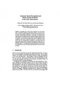
During search we deal with hypotheses which associate phonemes with segments; these A i segments can be referenced by their boundary positions [ti−1 , ti ]. Up till now we set no restrictions on these ti -s except the trivial ones (they are integer values in increasing order, 1 ≤ t i ≤ t). We may, however, define a set T and allow only its elements; this T is called the set of possible segmentations, and the method which computes T is called the segmentation algorithm. Indeed, it is very unlikely that every value between 1 and t will be needed, but keeping unused values in T makes the search process more time-consuming and without any gain. Also, this T in the ideal case coincides with the real boundary between phonemes, which can hopefully be predicted via signal processing techniques [26]. The basic segmentation algorithm draws a possible bound at every kth frame, which is quite a dull, but satisfactorily-working method. Next we present three other methods, which all rely on a b i bound probability for every ai frame, supplied by an ANN trained in regression mode on the classic 13 MFCC ∆ coefficients. One may think that supplying the bi values solves the whole segmentation problem; pursuing this idea, the first two methods are straightforward ones. The Thresholding Algorithm still places a possible boundary at every k th frame, but only if the corresponding bi value exceeds a threshold pmin (see Figure 1). This method yielded poor results: parameter adjustments led to a 5

Figure 1: Above: the spectrum of a speech excerpt, along with its correct segmentation. Below: the same spectrum with the bi values and the output of the Thresholding Algorithm. Method Thresholding Thresholding Maximum Maximum LIF LIF Baseline

Parameters k = 6, p = 0.065 k = 6, p = 0.070 k=3 k=4 k = 6, p = 1.75 k = 7, p = 1.30 —

Correctness 96.06% 97.49% 93.90% 95.34% 97.85% 98.20% 96.42%

Accuracy 94.94% 95.70% 90.68% 92.83% 96.42% 95.69% 95.34%

Speed-up rate 110.83% 87.70% 78.29% 137.02% 155.57% 127.26% 100.00%

Table 4: Some results obtained using the Thresholding, Maximum and LIF algorithms on the Medical Database (sentence recognition, segment-based case), with their parameters. small speed-up, but the recognition figures became worse, while other configurations improved the accuracy, but caused some slow-down. These results are probably due to the fact that the change of spectrum (reflected by the bi values) often occurs over a long time with slightly higher b i values, which this method could not detect. Our second method, the Maximum Algorithm looks for positions where the bi values take their local maxima over a given interval. By adjusting the size k of the neighbourhood examined, we can set a minimal distance between the suggested boundaries (see Figure 2). Although this method seemed to be the most promising one, in practice it was not so: it inserted few needless bounds, but it also skipped some vital ones, which is a serious mistake. Furthermore, the algorithm was only limitedly tuneable with its single parameter being a small integer. The failure of these two methods suggests that a more complicated solution is needed. The LIF Algorithm seeks to dynamically adjust the density of possible bounds so that it is proportional to the local bi values. A solution for this is to apply a leaky integrate-and-fire (LIF) neuron model [6]. Its operation is simple: the neuron integrates its input until the sum reaches a certain threshold; then the neuron fires, its potential is reset, and the process starts again. It can be refined by making the integration “leaky”, so that the sum decays with a time constant. The model may also incorporate a refractory period, above which it is not excitable. In our segmentation algorithm the b i values are the input for the integrate-and-fire neuron: where these values are higher, their sum reaches the activation threshold sooner, so the spikes become more dense. The density of the spikes can be controlled by the 6

Figure 2: Above: the same spectrum as in Figure 1 with the bi values and the output of the Maximum Algorithm. Below: the same spectrum with the bi values and the output of the LIF Algorithm. threshold p, while by setting the refractory period k a minimum distance between the neighbouring spikes can be guaranteed (see Figure 2). This algorithm, unlike the others, achieved a satisfactory improvement in speed with no loss in accuracy; it was even able to raise the overall recognition scores and get a nice gain in speed (see Table 4). While the Maximum Algorithm was very good at finding possible phoneme bounds, it could not be tuned. The Thresholding Algorithm could be fine-tuned with its two parameters, but the method itself was too primitive. The LIF algorithm, however, seems to be the golden mean between the two: it has two parameters for tuning, suggests phoneme bounds at smarter places than the Thresholding Algorithm does, and it takes the context into account.

Summary of Theses I/1. The author created a multi-pass search technique to speed up the search process in speech recognition. This method was based on the use of multiple, hierarchical phoneme sets, which were created by clustering the elements of the original phoneme set based on the confusion matrix of phoneme classification. Using the hierarchical property of the phoneme groups, the corresponding passes can be readily implemented as a more compact phoneme group unites several. This way the search process was significantly speeded up (published in [13; 14; 25]). I/2. The author constructed a method for detecting the interchange of phonemes to more precisely model the bound between them. Based on it, he constructed a novel algorithm to supply a set of possible phoneme boundaries. As shown by the results, this algorithm can indeed lead to a significant speed-up over that of the standard segmentation method, which was our aim. Moreover, a careful configuration of this method also gave a noticeable improvement in the recognition accuracy along with a significant speed-up (published in [18]). I/3. The author examined the behaviour of the multi-stack decoding algorithm and the Viterbi beam search method. These algorithms both store a number of hypotheses for each possible bound between phonemes. By introducing a number of techniques to more cleverly adjust the number of hypotheses stored, the author was able to speed up the search process along with little or no loss in the recognition accuracy (published in [11; 12; 14; 16; 25]). 7

2

Improving the Accuracy of Speech Recognition

In the second part we seek to make the speech recognition process more accurate: we inspect areas which could lead to an improvement in the recognition accuracy. As there are a large number of areas which might be able to do this, we had to restrict our scope to just a few such areas. We will concentrate on the application of different aggregation operators in hypothesis cost calculation and on the so-called anti-phoneme problem, as these have practically no additional time requirements.

2.1

Using Aggregation Operators to Calculate Hypothesis Probabilities

Recall that in the discriminative approach we want to find the most probable word w ˆ ∈ W for which P (A|w)P (w) is maximal. Concentrating on the former factor we will decompose it into P (A|w) =

n Y

P (Aj |oj ),

(8)

j=1

where the word w equals its phoneme sequence o1 , . . . , oj , and A = A1 , . . . , An is the decomposition of the speech signal A = a1 , . . . , at for non-interleaving segments, one for each phoneme. This formula is based on the assumption of independence; but it was shown [31] that this assumption is actually false, and the use of other operators is also viable as they may fit the actual problem better than the default multiplication. This allows us to use a more general representation [29], namely
P (A|w) = g2 P (A1 |o1 ), P (A2 |o2 ), . . . , P (An |on ) , (9) where g2 is an operator used to construct word-level probabilities from phoneme-level ones. Following this line, another operator (g1 ) is used to supply the phoneme-level P (Aj |oj ) values from local information sources. In a typical frame-based environment (as in the case for a Hidden Markov Model (HMM)), g1 is usually based on the aj frames and is defined as P (Aj |oj ) = g1 (Aj , oj ) = g1 (atj−1 , . . . , atj , oj ) =

tj Y

t −tj−1

cojj

· P (al |oj ),

(10)

l=tj−1

where coj is the state self-transition probability for the state belonging to phoneme o j , and typically a Gaussian Mixture Model (GMM) supplies the P (al |oj ) values. In a segment-based case g1 is usually the length-normalized output of the phoneme classifier [29]. In the following we will change either the g1 or g2 operator. This way the probability of word-segment pairs is affected, which can also change the most probable one, preferably improving the accuracy, which was our aim. 2.1.1

Using Mean Aggregation Operators

First we opted for an operator whose behaviour could be tuned between different extremes. It led us to the mean aggregation operators taken from fuzzy logic [23], namely the root-power mean operator [4] Gα (x1 , . . . , xj ) =



xα1 + . . . + xαj j

 α1

,

α ∈ R.

(11)

It is well-known [20] that when α → −∞, Gα → min(x1 , . . . , xj ); G−1 equals the harmonic mean; 8

Operator used Nothing (baseline) Gα Gα,λ with λ = 0.7 Gα,λ with λ = 0.8 Gα,λ with λ = 0.9 Gα,λ with λ = 1.0

α – 0.6 0.4 0.5 0.5 0.6

Accuracy 77.83% 84.35% 83.04% 83.91% 84.78% 84.35%

Table 5: The best accuracies for the root-power mean operator and for the decaying root-power mean operator on the Children Database (isolated word recognition, segment-based case). Operator used Nothing (baseline) Gα as g1 Gα as g2

α as g1 – 0.94 0.94

α as g2 – – 1.00

Accuracy 94.20% 95.13% 95.13%

Table 6: The best accuracies for the root-power mean operator on the Telephone Database (isolated word recognition, frame-based case). First the α for g1 was optimized, then we set the α for g2 too. when α → 0, Gα tends to the geometrical mean; G1 equals the arithmetical mean; and when α → ∞, Gα → max(x1 , . . . , xj ). By varying the α parameter we can make a continuous transition from minimum to maximum, which means that this operator is quite flexible, coming in handy in any application. Now we define a variant of this operator, the decaying root-power mean operator, by Gα,λ (x1 , . . . , xj ) =

λj−1 xα1 + λj−2 xα2 + . . . + λxαj−1 + xαj j

! α1

,

(12)

where α ∈ R as before and λ ∈ [0, 1] is a weighting parameter used to make the last value more important than the ones before it. In our case the last value refers to the last phoneme or frame of the hypothesis, so this operator seems to be a good variant for our particular problem. Next we seek to utilize these operators either as g1 or g2 , which requires setting their parameters. The root-power mean operator can be optimized quite easily with its single parameter: first an interval was determined by preliminary tests where it worked adequately, then this interval was explored with a small step size. For the decaying root-power mean operator, however, we chose a number of λ values, and then the remaining parameter (α) could be set in the same way as before. In the segment-based case, of course, only g2 can be changed as here g1 is not a true operator. Table 5 shows the best accuracies and the corresponding α parameters for the root-power mean operator Gα and for the decaying root-power mean operator Gα,λ for different λ values. Utilizing Gα led to a big improvement in the recognition accuracy, indicating that perhaps it models the problem better than the default multiplication; but later, the decaying root-power operator achieved only a slight improvement, which suggests that here it has no real advantages over G α and it is also a more complex one. In the frame-based case, however, it was possible to modify both operators. For the sake of easier usage we did not set their parameters in parallel, but first optimized g 1 , leaving g2 in its basic, multiplication form; then we turned to g2 , keeping g1 as the optimized operator (see Table 6). We found that setting g1 led to a significant improvement, but changing g2 led to no further gain.

9

t-norm family Best accuracy Rel. error reduction

TP 92.17% 0.00%

TL 0.26% —

TλSS 93.47% 16.60%

TλH 92.60% 5.49%

TλY 89.45% —

TλD 93.47% 16.60%

TλAA 93.04% 11.11%

Table 7: Recognition percentage scores and relative error reduction rates for the standard triangular norms applied on the Children Database (isolated word recognition, segment-based case). t-norm family Best accuracy Relative error reduction Best correctness Relative error reduction

TP 91.69% 0.00% 92.03% 0.00%

TL 0.69% — 0.81% —

TλSS 92.61% 11.07% 93.31% 16.06%

TλH 92.50% 9.74% 93.19% 14.55%

TλY — — — —

TλD 92.25% 6.73% 93.03% 12.54%

TλAA 92.03% 9.74% 92.73% 8.78%

Table 8: Accuracy and correctness values and relative error reduction rates with the standard triangular norms applied on the Medical Database (sentence recognition, segment-based case). 2.1.2

Using Triangular Norms

Practically any kind of operator can be used either as g 1 or as g2 , but only a small fraction of these operators could work well. Moreover, we should use operators which can be easily applied and fine-tuned, so we set two criteria: their behaviour should be easily modifiable (having one or more parameters), and, as the default operator is the product one, they should be “multiplication-like”. The triangular norms are standard operators of fuzzy logic [4; 23], and they fulfil both requirements, thus we applied them. Another reason for using t-norms is that in fuzzy logic they represent AND-like relations, and here we also have AND-connections (i.e. segment A 1 is phoneme o1 with x1 probability AND segment A2 is phoneme o2 with x2 probability etc.). Definition 1 A function T : [0, 1]2 → [0, 1] is a triangular norm (t-norm) if and only if: (T1) T (1, x) = x (T2) T (x, y) = T (y, x) (T3) T (x, y) ≤ T (u, v)

for all x ∈ [0, 1], (boundary condition) for all x, y ∈ [0, 1], (commutativity) for any 0 ≤ x ≤ u ≤ 1, (T is nondecreasing 0 ≤ y ≤ v ≤ 1, in both arguments) (T4) T (x, T (y, z)) = T (T (x, y), z) for all x, y, z ∈ [0, 1]. (associativity) It is easy to see that the product operator is also a t-norm, so we will refer to it as T P . And Definition 2 A t-norm T is said to be continuous Archimedean

if T as a function is continuous on [0, 1]; if T (x, x) < x for all x ∈ (0, 1).

As these two properties seem to be important for a function used either as g 1 or g2 , we will use triangular norms which fulfil both these requirements. A number of well-known triangular norms described by Klement, Mesiar and Pap [23] were tested. A triangular norm is a two-operand function, and (either as g1 or g2 ) we need an operator which can handle any number of arguments, but it can be easily resolved by the associativity property ((T4)). All the norms tested have one parameter (except the Lukasiewicz norm TL , which has none), giving them the required flexibility, but still remaining 10

easy to set (which was done in the same way as that for the root-power mean operator). The standard triangular norms were tested in a segment-based context only, applied as g 2 , but both in an isolated word recognition task (see Table 7) and in a sentence recognition one (see Table 8). We could achieve a nice reduction in the error rates, depending on the actual standard triangular norm applied. 2.1.3

Using a Two-Parameter General Triangular Norm

In the next step we seek to apply something more general than the standard triangular norms. Dombi introduced a generalized family of triangular norms, which can be represented in the following way: (α)

TGD,γ =

1 1 + Dγ (x)

α > 0,

where Dγ (x) =

1 γ

n  Y i=1

1+γ



1 − xi xi

α 

−1

(13) !!1/α

(14)

and γ > 0 [3]. Furthermore, this operator includes many well-known and widely-used triangular norm families (like the Dombi, Hamacher, Einstein and the product operators) as some special cases. Its application required some adaptation for the setting of parameters, as it has two (α and γ) instead of the standard triangular norm families which had only one (λ). As α and γ have to be set in parallel, the methods used previously cannot be applied. One way could be the determination of an adequately working interval for both parameters by preliminary tests, which intervals could be explored by some step sizes; but this method raises the number of tests needed to the second power. We followed another line of thinking: by fixing all the possible settings of a speech recognizer configuration except the parameters of the triangular norm, the accuracy can be considered as a function of these two parameters, which is to be maximized. In our case, where only g 1 or g2 is changed, it is an optimization problem in a two-dimensional space, and was solved by utilizing a gradient-based optimization method: the SNOBFIT package [21]. The experiments were done in a frame-based context, replacing g1 and keeping g2 at its multiplication, in a sentence recognition task. We allowed 500 iterations, which is a fraction of the number of tests required by the first strategy. The error rates were greatly cut (see Table 9): a relative error reduction of above 50% was achieved, which is a much better score than what could be achieved by using a standard triangular norm. 2.1.4

A More General Approach: The Logarithmic Generator Function

Now we shall present a more general way of modelling triangular norms, and supply an applicationoriented technique to fit it to the given problem. For this we first have to state another definition. Theorem 1 A t-norm T is continuous and Archimedean if and only if there exists a strictly decreasing and continuous function f : [0, 1] → [0, ∞] with f (1) = 0 such that
T (x, y) = f (−1) f (x) + f (y) ,

where f (−1) is the pseudo-inverse of f defined by ( f −1 (x) if x ≤ f (0) f (−1) (x) = 0 otherwise. 11

The n-ary extension of this formula is trivially T N (p1 , p2 , . . . , pN ) = f −1

X i

 f (pi ) .

(15)

This representation is unique up to a positive multiplicative constant. If the t-norm is strictly monotonously increasing, then f is strictly monotonously decreasing, and the pseudo-inverse function f (−1) is the normal inverse f −1 . We will apply this case; then f is an additive generator of T [4]. Now we can turn to its application. In a typical speech recognition environment, to avoid underflowing, instead of a probability p we use the cost c = − log p. Since it is desirable not to convert cost to probability and vice versa all the time, we first incorporate this conversion into Eq. (15), i.e. N  X  − log f −1 f (e−ci ) .

(16)

φ(x) = f (e−x ).

(17)

i=1

As we always apply this formula, it is straightforward to include the calculation of the negative exponential into f ; i.e. we will define the logarithmic generator function as

Now we can incorporate φ(x) into Eq. (16); that is, φ−1

N X i=1

N   X  φ(ci ) = − log f −1 f (e−ci ) = − log T (e−c1 , e−c2 , . . . , e−cN ),

(18)

i=1

so using the logarithmic generator function φ(x) in the same way as the additive generator function f (x) will lead to the calculation of the same triangular norm T , only with cost values instead of probabilities, both as arguments and as the result. The logarithmic generator function is φ(x) : [0, ∞] → [0, ∞], is strictly increasing, φ(0) = 0, and is unique up to a multiplicative constant for a given T t-norm. To model φ(x) practically any approximation could be used; our solution assumes that 1 ,...,mn it is piecewise linear. Let φ = φm a1 ,...,an : [0, ∞] → [0, ∞] be a piecewise linear, strictly increasing function with break points on the domain as 0 = a0 < a1 < a2 , . . . , an < an+1 = ∞ and with steepness values m1 , m2 , . . . , mn > 0 respectively and mn+1 = limx→∞ φ0 (x) = 1. That is, φ(x) = (x − aj )mj+1 +

j X

(aj − aj−1 )mj , aj ≤ x < aj+1 .

(19)

i=1

The function φ is unique up to a positive multiplicative constant; by setting m n+1 to 1, we fix one of these equivalent representations. Furthermore, we can position these control point a j -s at values where they represent our problem as accurately as possible; so, for given control points, a function φ can be described by the vector of the n steepness values (m = (m 1 , m2 , . . . , mn )). The only remaining issue is the choice of control points, for which we suggest a statistic of use: we noted that, during a typical recognition, which cost values had to be handled. The resulting histogram was divided into n + 1 equal parts, the boundaries being the a i values (see Figure 3). This way, fixing the value of n, setting the control points, and optimizing m for maximum accuracy, we can easily model the logarithmic generator function and so the triangular norm itself. Table 9 shows the performance of this method in a frame-based context (so g 1 was changed while g2 remained multiplication): using the logarithmic generator resulted in the best performance, but only if n was big enough to give the norm the required flexibility. And, as the logarithmic generator works directly on the cost values, it was the easiest one to apply. 12

4

8

x 10

6

4

2

0 0

10

20

30

40

50

60

−log p

Figure 3: A histogram of the − log p values appearing during a standard speech recognition process using multiplication, in the interval [0, 60], with the suggested positioning of n = 8 control points. Method Product (baseline) Dombi t-norm Generalized Dombi operator t-norm via logarithmic generator, n = 8 t-norm via logarithmic generator, n = 16

Accuracy 96.76% 97.57% 98.49% 98.27% 98.84%

Correctness 98.38% 98.84% 98.95% 98.84% 99.19%

Sentences 92.66% 93.33% 94.66% 94.00% 96.00%

Table 9: The best accuracy and correctness values obtained for the triangular norms tested on the Medical Database (sentence recognition task), frame-based case, and the ratio of correct sentences.

2.2

The Anti-Phoneme Problem

Finally we will focus on the anti-phoneme problem, arising in a segment-based context only. Its purpose is to decide whether speech segments correspond to a “real” phoneme or not, for which we have a large number of examples for correct segments in the form of a hand-labelled corpus, but there is no sure way of having counter-examples since these should contain anything else occurring in a sound recording (noise, segments longer or shorter than one phoneme, etc.) called “anti-phonemes” [7]. As we only have examples of the positive class, it is an example of one-class classification [28]. Recall that in the speech recognition problem we look for the most probable word w ˆ∈W w ˆ = arg max P (A|w)P (w). w∈W

(20)

Concentrating on P (A|w), we assume that the A signal can be divided into non-overlapping segments. Since this correct segmentation of the signal is not known, it appears as a hidden variable S: P (A|w) = arg max P (A, s|w). s∈S

(21)

There are several ways of decomposing P (A, s|w) further, depending on our modelling assumptions, as S is not well-defined at this point. As the segments are assumed to be independent, the corresponding local probability values will simply be multiplied. For example, in our system we apply [30] n Y P (oj |Aj )P (α|Aj ) , P (oj )

(22)

j=1

where the anti-phoneme is denoted by α, thus P (α|Aj ) denotes the probability that the given segment is not an anti-phoneme. Next we will focus on methods for estimating the P (α|A j ) probability value to improve the recognition accuracy. 13

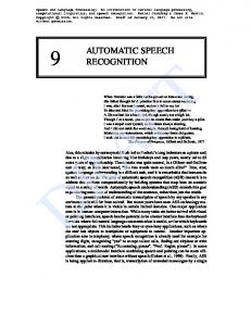
Figure 4: Some generated counter-examples with different settings. Left to right: 1st: (dist, curv) = (1, 0), 2nd: (dist, curv) = (0.4, 0), 3rd: (dist, curv) = (1, 0.5), 4th: (dist, curv) = (1, 1). curv = 0 generates points of a hyperplane, while curv > 0 generates points of a better fitting hyper-surface; dist controls the distance between the boundary points and the generated counter-examples. There are two main approaches for solving a one-class classification problem like this. First, we could use a method which can by itself model all the positive examples. The second approach is to take the actual occurrences of phonemes as positive examples, and generate anti-phonemes as negative ones; then the two classes can be separated by some statistical method like ANNs. Of course this automatic generation is not straightforward, and it can also be done in two ways: task-specifically, or by using some general algorithm. Perhaps the most straightforward way of describing all the phonemes is to model them with the sum of some Gaussian curves. And this is essentially what Gaussian Mixture Models (GMMs) [5] do, hence their application is the default solution in the literature [7]. On the other hand, T´oth introduced a method for generating “incorrect” segments [30]. This algorithm, called “Incorrect Segment Sampling”, is based on the idea that the negative examples are probably parts of speech which start and/or end at positions where there is no real bound between phonemes. If we know the real phonetic boundaries – which is the case for any training database –, then we can generate negative examples by choosing incorrect phoneme boundaries for the start and/or end segment bound. The actual solution is quite straightforward: for each phoneme several anti-phonemes are generated by placing one or both phoneme boundaries earlier or later by δ milliseconds. Besides applying a speech recognition-specific method, we can also use a general counter-example generation algorithm, with the set of positive examples X as its input and a set of negative or counterexamples as its output. B´anhalmi introduced one such counter-example generation algorithm [2], which we applied for the anti-phoneme task as the third method. The main idea behind this algorithm is to project each positive example point x ∈ X outside X. To do this, first the set B of the boundary elements of X is calculated, then each positive example is transformed over the closest boundary point with the use of two parameters: curv controls the curvature of the resulting surface, while dist sets the distance of the resulting point from the appropriate boundary point. Finally the resulting point 14

Method GMM with 20 Gaussians Incorrect Segment Sampling General C.E., curv = 0.0, dist = 1.5 No anti-phoneme modelling

Accuracy 91.12% 91.97% 95.58% 88.17%

Correctness 91.80% 92.62% 95.82% 88.53%

Table 10: Some notable test results for all three methods on the Medical Database (sentence recognition, segment-based case). is checked to see whether it is an outer point of the original positive examples, which is done in the same way as the boundary points were identified. If it is not a real outer point, then the process has to be repeated with the second-closest boundary point, etc. This is done for each element of X, resulting in N negative examples for N positive ones (see Figure 4). This method has an obvious weakness: its time requirement for larger databases is very high. As in our case there were indeed large datasets, we had to deal with this issue. It meant that executing this algorithm with different dist and curv parameters took rather a long time. To solve this problem – which was essential for the practical use of this algorithm – we introduced a number of modifications. • We noticed that this algorithm could be divided into two distinct parts: the first one calculates the boundary points, while the second one is responsible for the actual counter-example generation. Fortunately the first one is responsible for the higher time complexity; the dist and curv parameters, however, appear in the second part only. Thus, no matter how many parameter combinations we seek to test, the first – and much slower – part has to be computed just once. • This second part could be divided up still further: when we know the elements of the boundary set, for each element x first we have to find the closest boundary point x b ∈ B. This procedure also has nothing to do with the varying parameters, so it can be separated from the actual projection and should also be computed just once (although strictly after determining the boundary elements), then its result can be stored. Thus, when trying out a new dist and curv parameter value pair, we only have to read the index of the closest boundary instead of calculating it again as was done in the original version of this algorithm. • Next we found that the last part where we test whether the resulting point is an outer point is also not necessarily needed: for larger dist values (in our case dist ≥ 1.5) the projected point lies too far away from the original example set to be an inner point. Of course the smaller the dist value is, the more likely that some of the projected points may be inner points, but this risk is acceptable because omitting this part leads to an overwhelming speed-up. Using these modifications it became possible to test all three methods on a sentence recognition task (see Table 10); the features were the same as those used for phoneme classification. For the baseline value we did not use any anti-phoneme model at all. The general counter-example generator method proved to be the most successful one, but it could not have been applied without the modifications introduced, as it would have been practically impossible to set its two parameters satisfactorily due to the CPU time requirements.

15

I/1. I/2. I/3. II/1. II/2. II/3.

[13] [18] [16] [11] [12] [14] [25] [15] [24] [10] [17] [9] • • • • • • • • • • • • • • • • •

Table 11: The relation between the theses and the corresponding publications

Summary of Theses II/1. In the search task of speech recognition the generated hypotheses are ranked by their cost values, usually calculated in two steps: first phoneme-level costs are aggregated from the frame-level ones, then the cost of the hypothesis is calculated from the phoneme-level values. The author applied a number of fuzzy functions at these levels: mean aggregation operators and triangular norms were tested to improve the recognition accuracy. He also modified the root-power mean operator by introducing a weighting parameter to make earlier observations less important. Furthermore, to set the two parameters of a generalized triangular norm, he turned the problem into a minimization one in a two-dimensional space and applied a global optimization method. The improvements in accuracy indicate that these operators fit the problem better than default multiplication (published in [10; 12; 14; 15; 24; 25]). II/2. The author proposed an application-oriented method for modelling triangular norms by introducing the logarithmic generator function. Assuming that this function was piecewise linear, he introduced a technique to adequately fit it to the actual application based on the histogram of the occurring probabilities. He applied this method in the speech recognition minimization problem introduced in Thesis II/1, and showed that it can improve the performance by a greater amount than any other classical norms tested (published in [17]). II/3. The author applied a general counter-example generator method from the literature in the anti-phoneme problem of segment-based speech recognition. To make it possible to use he also introduced several modifications to this method, which were essential to reduce its time requirement. Doing this, he was able to markedly reduce the error rates of the speech recognition system, even when compared to other standard solutions for this problem (published in [9]).

Conclusions In the author’s opinion the most important aspects of speech recognition are accuracy and speed, as we have to recognize the speech signal uttered as accurately as possible, and possibly within real time. He sought to introduce improvements for both, and it resulted in a number of techniques which, based on the results of the experiments, proved to be successful. Most methods have parameters which, of course, probably have to be set again in a different environment, but the test results described here confirm the potential benefits of these methods. Some experiments led to some quite general techniques like the logarithmic generator function, and the refinements over the general counterexample generator algorithm, which could be applied in areas outside of speech recognition as well. 16

References [1] L. R. Bahl, P. Gopalakrishnan, and R. L. Mercer. Search issues in large vocabulary speech recognition. In Proceedings of the 1993 IEEE Workshop on Automatic Speech Recognition, Snowbird, UT, 1993. [2] A. B´anhalmi, A. Kocsor, and R. Busa-Fekete. Counter-example generation-based one-class classification. In Proceedings of ECML, pages 543–550, 2007. [3] J. Dombi. Towards a general class of operators for fuzzy systems. IEEE Transaction on Fuzzy Systems, 16(2):477–484, 2008. [4] D. Dubois and H. Prade. Fundamentals of Fuzzy Sets. Kluwer Academic Publisher, 2000. [5] R. O. Duda and P. E. Hart. Pattern Classification and Scene Analysis. Wiley & Sons, New York, 1973. [6] W. Gerstner and W. M. Kistler. Spiking Neuron Models. Cambridge University Press, 2002. [7] J. R. Glass. A probabilistic framework for segment-based speech recognition. Computer Speech and Language, 17(2):137–152, 2003. [8] G. Gordos and G. Tak´acs. Digital Speech Processing (in Hungarian). M˝uszaki K¨onyvkiad´o, 1983. [9] G. Gosztolya, A. B´anhalmi, and L. T´oth. Using one-class classification techniques in the antiphoneme problem. In Proceedings of the 2009 Iberian Conference on Pattern Recognition and Image Analysis (IbPRIA), volume LNCS 5524, pages 433–440, Porto, Portugal, 2009. [10] G. Gosztolya, J. Dombi, and A. Kocsor. Applying the Generalized Dombi Operator family to the speech recognition task. Journal of Computing and Information Technology, 17(3):285–293, 2009. [11] G. Gosztolya and A. Kocsor. Improving the multi-stack decoding algorithm in a segment-based speech recognizer. In Proceedings of the 16th International Conference on Industrial and Engineering Applications of Artificial Intelligence and Expert Systems (IEA/AIE), volume LNCS 2718, pages 744–749, Loughborough, England, UK, 2003. [12] G. Gosztolya and A. Kocsor. Aggregation operators and hypothesis space reductions in speech recognition. In Proceedings of the 2004 Conference on Text, Speech and Dialogue (TSD), volume LNCS 3206, pages 315–322, Brno, Czech Republic, 2004. [13] G. Gosztolya and A. Kocsor. A hierarchical evaluation methodology in speech recognition. Acta Cybernetica, 17(2):213–224, 2005. [14] G. Gosztolya and A. Kocsor. Speeding up dynamic search methods in speech recognition. In Proceedings of the 18th International Conference on Industrial and Engineering Applications of Artificial Intelligence and Expert Systems (IEA/AIE), volume LNCS 3533, pages 98–100, Bari, Italy, 2005. 17

[15] G. Gosztolya and A. Kocsor. Using triangular norms in a segment-based automatic speech recognition system. International Journal of Information Technology and Intelligent Computing (IT & IC) (IEEE), 1(3):487–498, 2006. [16] G. Gosztolya, A. Kocsor, L. T´oth, and L. Felf¨oldi. Various robust search methods in a Hungarian speech recognition system. Acta Cybernetica, 16(2):229–240, 2003. [17] G. Gosztolya and L. L. Stach´o. Aiming for best fit t-norms in speech recognition. In Proceedings of the 2008 International Symposium on Intelligent Systems and Informatics (SISY) (IEEE), pages 1–5, Subotica, Serbia, Sept 2008. [18] G. Gosztolya and L. T´oth. Detection of phoneme boundaries using spiking neurons. In Proceedings of the 2008 International Conference on Artificial Intelligence and Soft Computing (ICAISC), volume LNCS 5097, pages 782–793, Zakopane, Poland, 2008. [19] D. J. Hand, H. Mannila, and P. Smyth. Principles of Data Mining. The MIT Press, 2001. [20] G. H. Hardy, J. E. Littlewood, and G. P´olya. Inequalities. Cambridge University Press, 1968. [21] W. Huyer and A. Neumaier. Snobfit – stable noisy optimization by branch and fit. ACM Transactions on Mathematical Software, 35(2):1–25, 2008. [22] F. Jelinek. Statistical Methods for Speech Recognition. The MIT Press, 1997. [23] E. P. Klement, R. Mesiar, and E. Pap. Triangular Norms. Kluwer Academic Publisher, 2000. [24] A. Kocsor and G. Gosztolya. Application of full reinforcement aggregation operators in speech recognition. In Proceedings of the 2006 Conference of Recent Advances in Soft Computing (RASC), Canterbury, UK, 2006. [25] A. Kocsor and G. Gosztolya. The use of speed-up techniques for a speech recognizer system. The International Journal of Speech Technology, 9(3-4):95–107, 2006. [26] T. N. Sainath. Acoustic landmark detection and segmentation using the McAulay-Quatieri sinusoidal model. Master’s thesis, MIT, 2005. [27] R. Schwartz, L. Nguyen, and J. Makhoul. Multiple-pass Search Strategies, chapter 18, pages 429–456. Kluwer Academic Publisher, Philadelphia, PA, 1996. [28] D. M. Tax. One-class classification; Concept-learning in the absence of counter-examples. PhD thesis, Delft University of Technology, 2001. [29] L. T´oth, A. Kocsor, and J. Csirik. On Naive Bayes in speech recognition. International Journal of Applied Mathematics and Computer Science, 15(2):287–294, 2005. [30] L. T´oth, A. Kocsor, and G. Gosztolya. Telephone speech recognition via the combination of knowledge sources in a segmental speech model. Acta Cybernetica, 16(4):643–657, 2004. [31] S. Young. Statistical modelling in continuous speech recognition. In Proceedings of the International Conference on Uncertainty in Artificial Intelligence, Seattle, 2001. 18