overhead parallel performance monitoring, then, is to match the application monitoring demands to the effective operating range of the monitoring system (or ...
In Search of Sweet-Spots in Parallel Performance Monitoring Aroon Nataraj, Allen D. Malony, Alan Morris
Dorian C. Arnold, Barton P. Miller
Department of Computer and Information Science University of Oregon, Eugene, OR, USA
Computer Sciences Department University of Wisconsin, Madison, WI, USA
{anataraj, malony, amorris}@cs.uoregon.edu
{darnold, bart}@cs.wisc.edu
Abstract—Parallel performance monitoring extends parallel measurement systems with infrastructure and interfaces for online performance data access, communication, and analysis. At the same time it raises concerns for the impact on application execution from monitor overhead. The application monitoring scheme parameterized by performance events to monitor, access frequency and data analysis operation defines a set of monitoring requirements. The monitoring infrastructure presents its own choices, particularly the amount and configuration of resources devoted explicitly to monitoring. The key to scalable, lowoverhead parallel performance monitoring, then, is to match the application monitoring demands to the effective operating range of the monitoring system (or vice-versa). A poor match can result in over-provisioning (wasted resources) or in underprovisioning (lack of scalability, high overheads and poor quality of performance data). We present a methodology and evaluation framework to determine the sweet-spots for performance monitoring using TAU and MRNet.
I. I NTRODUCTION Post-mortem analysis of parallel application performance measurements has been the status quo for iterative performance diagnosis and tuning. However, the increased scaling of parallel systems argues for more online support for performance data access and processing. The importance of understanding parallel execution dynamics motivates the use of performance tracing, but scale amplifies trace size and analysis complexity. In contrast, profiling methods lose insight on temporal performance variation, which could prove to be important for identifying patterns of performance inefficiency. From the standpoint of adaptive parallel programs, neither conventional profiling nor tracing measurement, per se, provide adequate support for performance-driven dynamic tuning. Parallel performance monitoring extends parallel measurement systems with infrastructure and interfaces for online performance data access, communication, and analysis. Use of performance monitoring immediately raises concerns for the impact on parallel application execution from monitor overhead. Whereas the cost/benefit value of monitor use is ultimately determined by user requirements, innovations in scalable monitoring technology seek to reduce overhead impact by allocating additional physical computing resources for monitor deployment. The Supermon [1] and MRNet [2] systems can both operate in this manner. Integration of a parallel performance measurement facility with a monitoring
framework built on supplemental resources can deliver effective performance monitoring capability at large scale, as we demonstrated with the TAU Performance System and both Supermon [3] and MRNet [4]. What does it mean to be effective in the context of a parallel applications performance monitoring needs? The monitoring scheme chosen (e.g., performance events to monitor, access frequency, data analysis operation, and location of monitor consumer) are rightly determined by application semantics. For instance, many parallel scientific applications are both iterative in nature and phase based. Ascertaining how application performance changes from iteration to iteration relative to phases would naturally define a set of monitoring requirements. The problem is determining whether these requirements conflict with acceptable levels of monitor cost. The monitoring system presents its own choices, particularly the amount and configuration of resources devoted to the monitoring infrastructure. These choices result in a monitoring system with certain operational performance characteristics which translate into ranges of practical use. The key to scalable, low-overhead parallel performance monitoring, then, is to match the application monitoring demands to the effective operating range of the monitoring system (or vice-versa). A poor match can result in over-provisioning (wasted resources) or in under-provisioning (lack of scalability, high overheads and poor quality of performance data). We present a methodology and evaluation framework to determine the sweet-spots for performance monitoring with TAU and MRNet. In Section §II, the TAUoverMRNet (ToM) system for performance monitoring is described. The ineffective use of ToM based on naive requirements / configuration matching is demonstrated in Section §III. Following this, Section §IV presents a scheme for monitor bottleneck estimation. Section §V, using the estimation method, shows the relationship of monitor bottlenecks to performance data size and access frequency. This knowledge can help to characterize regions of effective monitor operation for different configurations and to guide good application choices for monitor use. Related work is given in Section §VI followed by conclusions and future work in Section §VII.
Back End
Streams
Co nt
Data
ro l --
>
MRNET Comm Node + Filter
TAU Front-End
>
l --
ro nt Co
Data
MRNET Comm Node + Filter
Fig. 1.
Back End
Streams
The TAUoverMRNet System
II. T HE TAUoverMRNet S YSTEM Scalable, online monitoring of parallel performance decomposes naturally into measurement and transport concerns. In TAU, an extensible plugin-based architecture allows composition of the underlying measurement system with multiple transports for performance data offloading. The ToM work explores the Tree-Based Overlay Network (TBON) model [5] provided by MRNet with an emphasis on programmability of the transport for the purpose of distributed performance analysis/reduction. The main components and the data/control paths of the system are shown in Figure 1. Back-End The ToM Back-End (BE) resides within the instrumented parallel application. The generic profile data offload routine in TAU is overridden by a MRNet adapter that uses two streams (data and control). The data stream is used to send packetized profiles from the application backends to the monitor. The offloading of profile data is based on a push-pull model, wherein the instrumented applications push data into the transport, which is in turn drained out by the monitor. The application offloads profile information at application-specific
points (such as every iteration) or at periodic timer intervals. The control stream is meant to provide a reverse channel from monitor to application ranks. ToM Filters MRNet provides the capability to perform transformations on the data as it travels through intermediate nodes in the transport topology. ToM uses this capability to distribute statistical performance analyses traditionally performed at the sink, in the process reducing the amount of performance data that reaches the monitor. One such filter performs distributed histogramming, with a histogram per profile event reaching the front-end at every monitoring interval. As an example, Figure 2 plots the Allreduce event’s cumulative runtime retrieved as histograms at every iteration. The data is from a run of the FLASH [6] application’s 2-D Sod problem on 1024 processors of the LLNL Atlas cluster. The view allows tracking both temporal and spatial patterns in the event’s performance. ToM provides these performance views in a scalable and low-overhead fashion. For instance, in monitored runs of the FLASH 2-D Sod problem, weak-scaling from 64 to 512 processors, with performance data offload occurring every
iteration, the total overhead from measurement and transport amounted to less than 1% of uninstrumented runtime [4]. FLASH Sod 2-D | Event: Allreduce | N=1024
No. of Ranks
18
350 300
Total Event Runtime (secs)
15
250
12 200 9 150 6 100 3
50
0
0 50
Fig. 2.
75
100 Application Iteration #
125
150
Allreduce Observations from Distributed Histogram Filters
Front-End The ToM front-end (FE), the root of the transport tree, invokes the MRNet API to instantiate the network and the streams. In the simplest case, the data from the application that is transported as-is, without transformations, is unpacked and written to disk by the FE. More sophisticated FEs (that are in turn associated with special ToM filters) accept and interpret statistical data including histograms and functionally-classified profiles. III. NAIVE M ONITORING C HOICES We motivate the need to make informed monitoring choices through example runs where choices are made without regard to monitoring system capability resulting in unfavorable outcomes. The ideal solution is one in which the application monitoring requirements and monitoring system operating parameters are well matched. Such a system must allow the overhead caused to the application due to monitoring to be determined and controlled and provide for global (spatial and temporal) consistency in the monitored performance views. A globally consistent view includes all of the ranks’ data (spatial) with all of the data being drawn from the same monitoring interval (temporal). We restrict ourselves to overheads related to the offload and transport of performance data (measurement related overheads are outside the scope of the current work). Assuming a SPMD application model, the set of monitoring choices in the application reduces to the monitoring offload interval and the profile event count. Fixing the event count (to 64 profile events), we focus on the effect of offload intervals. A simple bspbench benchmark that models bulk-synchronous processing (BSP) busy loops over a calibrated work loop to match the requested computation time. It then executes a barrier followed by a profile offload. This sequence is repeated for the configured number of iterations. Since an offload occurs every iteration, the offload interval matches the compute time per iteration. ToM is configured with a statistics filter that
produces summary statistics (such as mean, standard deviation, min, max) for each event across the ranks. In the following experiments the bspbench is configured to use 64 application ranks (N), 64 profile events (E), 1000 iterations (I) and the offload intervals of 100, 24 and 6 ms. ToM is constructed with a fanout (FO) of 8. For every iteration the maximum time spent within the offload operation across the ranks is reported as the Offload Cost (OC) and represents the direct cost to the application from performing the offload. The maximum time between the start of an offload operation at a BE and the arrival of the single, reduced profile at the FE is reported as the One Way Delay (OWD). As the dumps are assumed to occur synchronously across the ranks, the OWD is calculated as the difference between the recv-time and the earliest send-time. TAU performs clock synchronization at startup across all application and ToM processors. Figure 3 (A) plots the OWD (bottom) and the OC (top) at every offload iteration for two cases (6ms and 100ms intervals). Examining the 100ms case first, we see that apart from a few small spikes, the OWD remains stable at about 60ms. Similarly its OC is stable and relatively low (2 to 4 ms). In contrast, the OWD in the 6ms case starts small but very quickly grows two orders of magnitude (to over 6000ms). The OWD then plateaus and exhibits a periodic pattern of growth followed by sudden drops. Associated with the sudden periodic drops are large spikes in the OC. This behavior can be explained by the fact that MRNet uses a tree of TCP connections as its underlying transport. Offloading at the rate of once every 6ms happens to be higher than the service capacity of the system resulting in queuing of the profiles in the path from BEs to FE. This queuing is reflected in large OWD values. As the queuing persists, buffer overflows occur at some point in the path (before or at the bottleneck). This triggers the TCP flow-control at the sender in the previous hop to stop forwarding, eventually causing that hop’s buffers to overflow as well. The back-pressure propagates all the way to the BE. The TCP flow-control at the BE causes the MRNetsocket send operation to block resulting in the large OC spike. Due to the blocked time, the application’s offload rate is temporarily lowered allowing the ToM system to catch up. But once buffers become available again, the application returns to its original offload interval leading to the repetitive pattern. The impact to the application follows directly from the blocked send operations (large OC spikes). Figure 4 plots the mean OC on the left-side axis for the three offload intervals as the curve labeled OC Blocking. These OC values represent overheads ranging from 2.4% (at 100ms) to 779.4% (at 6ms) of application runtime. While consistent global snapshots are being delivered, the choice of 6ms intervals leads to an excessive overhead level. Given that the overheads are attributable to the large blocking times, would a non-blocking offload solution help? The actual offload can be performed in a separate consumer thread with the main application thread placing the profiles into an unbounded buffer. This decouples the application from the actual offload and provides latency-
10000
Offload Cost (ms)
1000
100
10
1 Offload Interval: 6ms Offload Interval: 100ms
OWD (ms)
100000 10000 1000 100 10 0
100
200
300
400 500 600 Offload Iteration #
700
800
900
1000
(A) Blocking Offload
Offload Cost (ms)
10
1
0.1 Offload Interval: 6ms Offload Interval: 100ms
OWD (ms)
100000 10000 1000 100 10 0
100
200
300
400 500 600 Offload Iteration #
700
800
900
1000
(B) Non-blocking Offload Fig. 3.
Varying Offload Interval: Offload Cost (top), One Way Delay (bottom)
hiding. Figure 3 (B) plots the results from such a non-blocking scheme. The OC (top plot) of both configurations is relatively small and stable (since the actual offload is occurring in a worker thread). But the OWD of the 6ms case shows an early large growth followed by a continuous steady growth (unlike the plateau in (A)). The final OWD is in the range of 60000ms, an order of magnitude larger than the blocking case. This is attributable to the fact that in the absence of blocking experienced by the producer, there are no temporary rate reductions. As the curve labeled OC Non-Blocking in Figure 4 shows, the overhead goes from 1.8% (at 100ms) to 27.8% (at 6ms) of runtime. While 27.8% is still quite large,
it is a linear increase (of approx. 16 times) matching exactly the decrease in the interval. Unfortunately the non-blocking scheme does not fare much better. Figure 4’s right-side y-axis plots the Excess Data Reception Time which represents the extra time taken (after completion of the parallel application) to retrieve any remaining queued performance data. It took about 4.75 times longer to get the remaining data out resulting in an overall overhead of 607%. If performance data collection had stopped with application execution, only a few snapshots of the early iterations would have been retrieved. In both previous cases, the choice of certain monitoring intervals results in more profile offloads than the configured
100 Loss Occured | Interval: 6ms 90
48 40 % Global Snapshots Successfully Received
MPI Rank (# 0 - 63)
56
32 24 16 8 0 Loss Occured | Interval: 24ms
MPI Rank (# 0 - 63)
56 48 40 32
80
70
60
50
40
30
24 16
20 Offload Interval: 6ms Offload Interval: 24ms Offload Interval: 100ms
8 0 0
100
200
300
400
500 600 Offload Iteration #
700
800
900
1000
(A) Loss Maps
Blocking vs. Non-Blocking : Mean Offload Cost and Excess Data Reception Time 500
Mean Back-End Offload Cost [OC] (ms)
450
40
400
35
350
30
300
25
250
20
200
15
150
10
100
5
50
0
Fig. 4.
20
30
40
50 60 Offload Interval (ms)
70
80
90
100
Excess Data Reception Time [EDR] (% of Runtime)
OC Blocking OC Non-Blocking EDR Blocking EDR Non-Blocking
10
2 (Sim) Acceptance Threshold
4 (Sim)
Local Decisions : Non-blocking, Lossy Offload
50
0
1 (Sim)
(B) % Successful Global Offloads Fig. 5.
45
10 0 (Real)
0 110
Comparing Blocking vs. Non-blocking Offload Schemes
monitoring system can handle. Neither of the schemes attempt to reduce the number of offloads. Given that the application ranks (at the BEs) can locally detect spikes in the OC (in the blocking case) or a full-buffer (in the non-blocking case with bounded buffers), can the ranks then simply drop the profile that is yet to be offloaded? A lossy non-blocking scheme with bounded buffers results in such a local back-off policy. Figure 5 (A) provides a loss-map indicating the iterations at which specific ranks dropped profile offloads. In the both cases that had loses (24ms, 6ms) we see that loss affects the ranks unfairly, penalizing the same ranks repeatedly. Further, in the 24ms case, for almost every 8 application ranks there is one being victimized. It is no coincidence that the ToM fanout is 8. The structure is different in the 6ms case. Because of the losses, the % of globally consistent, complete profile offloads that could be generated was only 15% (24ms) and
11.4% (6ms) of the 1000 total iterations. In addition, all of the generated profiles were from the first 200 iterations. To improve upon this scheme by utilizing the structure seen in the loss map, one can define a loss Acceptance Threshold (AT) which allows an intermediate ToM filter to produce a reduced profile even when at most AT of its children fail to provide a profile. Figure 5 (B) plots the % global profiles generated from a simulation of this policy. At AT=0, the real data is plotted, with the simulated results at the other points. An AT=1 brings the 24ms case to almost 100% profile generation (since only one in every 8 experienced loss). But in the 6ms case this occurs only at an AT=4. The drawbacks of this approach arise from the inconsistent back-off signals that the application ranks receive and to which they react. With some ranks never being monitored and with no control over actual monitoring intervals, the result is a profile view at the FE that is inconsistent in both spatial and temporal aspects. The choices of 100ms, 24ms and 6ms intervals were made here knowing a priori that they were on either side of the system capacity. But they are intended to demonstrate the resultant behaviors when application monitoring choices (e.g. monitoring interval) and monitoring infrastructure choices (e.g. monitoring system resource allocation) are made independently without regard to each other. What is needed, then, is a way for the application (i.e. all its ranks) to determine the operating capacity of the ToM system as configured so as to consistently generate global profile views while staying within an acceptable overhead threshold. IV. E STIMATION OF B OTTLENECK I NTERVAL A global consensus across the application ranks regarding the operating capacity of the ToM monitoring system as configured, allows them to make informed, globally consistent decisions regarding performance profile offloads. Operating capacity refers to the number of profiles that the ToM system can handle per unit time without persistent backlogs for
One Way Delay [OWD] (ms)
350
Curr. OWD Rest. OWD + threshold Growth
300 250 200 150
termination, the High Interval at that point is instead returned as the BOI. Figure 6 shows the progress of one such search. Here the number of application ranks is 64, the ToM fanout (FO) is 8 and number of profile events is 64. The search parameters are set to l=20, k=2 with an error threshold of 2*restSD. At search step=0, the Curr. Interval is set to the initial High Interval (restOWD). The Low Interval is set based on the BOI for 32 profile events. In response to the Curr. Interval, the Curr. One Way Delay and growth remain below their thresholds. At step 2, the search then tries a lower offload interval, but finds that the Curr. OWD and growth shoot past their thresholds. This procedure continues until Step 9, when the range becomes smaller than the error threshold. Evaluating Estimation of Bottleneck Offload-Interval 15 Eval Metric [ { (Data Arrival Interval)*100/(Estimated Offload Interval) } - 100 ]
a given profile size and number of application ranks. The Bottleneck Offload Interval (BOI) metric is an estimator of the operating capacity of the system. It specifies the minimum possible interval between offloads that does not lead to queuing. This needs to be determined for different profile sizes of interest. When the application offload interval falls below the trueBOI of the system queuing must ensue and this queuing can be detected via the increasing One Way Delay values. Based on this we construct a binary-search where the search space consists of all possible intervals (from zero to infinity) and the comparison operator uses the OWD as a heuristic for guidance. To reduce the search-space to a manageable range, we first determine the upper bound (or the initial High Interval). We use a stop-and-go protocol with the BEs sending only after receiving acknowledgment from the FE that the previous round arrived. This ensures that no queuing occurs between rounds. The OWD measured in this phase (termed the Resting OWD or restOWD) is used as the initial High Interval. For the first search the initial Low Interval would be zero. For successive searches, performed in increasing order of profile size, the the BOI of the previous profile-size can serve as the initial Low Interval. In this resting phase, the standard deviation of the restOWD is also determined and used in the calculation of an OWD threshold (restOWD + k * restSD).
10
5
-10
100
N=64, FO=2 N=64, FO=4 N=64, FO=8
-20 % Change from Estimated Offload Interval Applied to Benchmark
-40
50 0
Fig. 7.
Offload Interval Estimation Evaluation
Offload Interval (ms)
65 60 55 50 45 40
Curr. Interval Low Interval High Interval 0
1
Fig. 6.
2
3
4 5 Search Step
6
7
8
9
Search Progress : Interval (bottom), OWD (top)
The main search phase starts by setting the Curr. Interval to the High Interval. The BEs synchronously send l rounds at the current interval. The FE calculates a growth metric based on the l OWD values. The growth (defined as the mean value of successive increases in OWD) captures increasing OWD trends. When growth > restSD and the mean-One Way Delay > OWD threshold, the Curr. Interval is set to the mid-point of the upper-half of the interval range and the Low Interval is moved up. Otherwise, Curr. Interval is set to the mid-point of the lower-half of the range and High Interval is reduced. This procedure continues until the interval range becomes less than an error threshold, satisfying the termination condition and returning the Curr. Interval as the BOI. If the growth was larger than the OWD threshold at
To evaluate the estimation we run the benchmark at progressively lower offload intervals than the estimated-BOI and measure the data arrival interval at the FE. In the case where the offload interval is larger than the true-BOI (which is not known), the data arrival interval should match the offload interval. But when offload interval is lower than the true-BOI, the data arrival interval should never drop below the trueBOI. The evaluation metric used is the % difference in the data arrival interval from the estimated-BOI. Figure 7 plots the evaluation metric resulting from offloading at intervals that are less than the estimated-BOI by 10, 20 and 40%. The curves for all three configurations never fall below +6% and instead begin to increase, suggesting that the estimated-BOI is at most within 10% of the true-BOI. ToM provides an API that informs the application of the BOI, OWD and OC for profile-sizes of interest to the application. The application, thus informed, can decide the granularity of profile offloads. For instance, an iterative application may determine that its iterations take 75 ms on average, but the estimated-BOI reported is 100 ms. It can then decide (consistently across the ranks) to drop every 4th profile offload, there by increasing its average offload interval (with the average taken over multiples of 4 rounds) to 100 ms, matching the
Bottleneck Offload Interval | N=8
Normalized SD (% Mean) of Rest. OWD (top) and Bott. Offload Interval (bottom) N=8, FO=2 N=8, FO=8
[OWD] FO=2 [OWD] FO=4 [OWD] FO=8
2048 1024
1
512 Bottleneck Offload Interval (ms)
Normalized SD of OWD
1.5
0.5
Normalized SD of Interval
0 [Interval] FO=2 [Interval] FO=4 [Interval] FO=8
3.5 3
256 128 64 32 16 8
2.5 2
4
1.5
2
1
1
0.5 0 16
32
64
128
16
32
64
256
128 No. of Profile Events
256
512
1024
256
512
1024
256
512
1024
(A) N=8
No. of Profile Events
Bottleneck Offload Interval | N=16
Fig. 8.
Stability of One Way Delay (top) and Offload Interval (bottom)
N=16, FO=2 N=16, FO=4 N=16, FO=16
2048 1024 512 Bottleneck Offload Interval (ms)
BOI. Further, by backgrounding the offloads (i.e. making them non-blocking), it can avoid potential backups due to burstiness from its lower-than-BOI short-term offload interval. The isolated nature of HPC resource allocations for jobs suggests a level of stability that may make BOI estimation at the start of every application run unnecessary. We performed five periodic probes (45 minutes apart) at varying fanouts and profile event sizes. Figure 8 plots the standard-deviations of both the OWD and BOI over the five probes. To be comparable, the standard-deviation is normalized and reported as a % of mean. Stability is observed across the configurations in both metrics. In such stable environments, the BOI estimates for a wide range of configurations can be generated, cached and reused for the length of time for which the stability is known to persist.
128 64 32 16 8 4 2 1 16
32
128 No. of Profile Events
(B) N=16 N=64, FO=2 N=64, FO=4 N=64, FO=8 N=64, FO=64
2048 1024
Bottleneck Offload Interval (ms)
512 256 128 64 32 16 8 4 2 1 16
32
64
128 No. of Profile Events
(C) N=64
Bottleneck Offload Interval The BOI estimation is performed over different profile sizes, starting at 16 events, increasing at power of two increments upto 1024 events. For each such configuration we determine the BOI, by picking the median of three trials. We begin with 8 applications ranks with ToM fanouts of 2 and 8. The filter performs the same summary statistics reduction as in previous experiments. Figure 9 (A) plots the BOI for the two N=8 configurations. What is immediately striking is
64
Bottleneck Offload Interval | N=64
V. C HARACTERIZING ToM P ERFORMANCE The Bottleneck Offload Interval estimation method and API provide the application the ability to discover the limits of monitoring system capability. The question yet to be answered is how to bridge monitoring requirements (as specified by both the user and application semantics) with the monitoring resource costs. Given an application size and the performance data reductions to be performed, what are the choices to be made with regards to ToM fanouts, monitoring offload intervals and number of profile events to sample? To help answer that, we characterize different ToM configurations using three metrics below.
256
Fig. 9.
Bottleneck Offload Interval Characterization
that the FO=8 curve performs better than the FO=2 curve at all profile sizes. At profile-size=16, there is a pronounced difference in the BOI values of the two configurations. As the profile size increases, FO=8 grows far more rapidly than FO=2. Since we are dealing with the BOI, queuing costs can
Overall and Direct Overheads of Offload | N=16, 64 N=16, FO=2 N=16, FO=4 N=16, FO=16 N=64, FO=2 N=64, FO=4 N=64, FO=8 N=64, FO=64
16 14
Overall Cost (ms)
12 10 8 6 4
Direct Cost (ms)
2 3.8
N=16, FO=2 N=16, FO=4 N=16, FO=16 N=64, FO=2 N=64, FO=4 N=64, FO=8 N=64, FO=64
3.3
2.8 16
32
Fig. 10.
64
128 No. of Profile Events
256
512
1024
BE Offload Costs: Direct (bottom) and Overall (top)
as the difference between the measured mean iteration runtime with offloads and the mean iteration runtime without offloads. OS buffering and variability in direct costs across the ranks (propagated globally at the barrier) explain the difference in the two costs. The Overall cost estimates application offload overhead. Limiting Transport Overhead Transport’s Limiting-Overhead | N=64 30
N=64, FO=2 N=64, FO=4 N=64, FO=8 N=64, FO=64
28 26 24 22 Limiting-Overhead (% Runtime)
be safely dismissed. Networking costs cannot account for the differences observed as in both configurations, the MRNet tree fits completely within a single (dual socket quad-core) node, with the application ranks occupying a second node. There are two primary costs associated with the reduction tree – reduction costs (TR ) and (de)packetization costs (TP ). The TR refers to the cycles required to perform a binary profile reduction operation. With N=8, a total of 7*TR cycles will be expended in reduction. The current statistics filter performs the reduction on the arrival of the last child’s profile. In the case of FO=2, the 7*TR reduction cycles are split across 7 processors, whereas in FO=8, a single thread performs all the reduction cycles. The TP is cycles required to pack an intermediate performance profile into a ToM packet (or unpack a packet into a profile data structure). For a fixed profilesize, TP is also fixed. But depending on the configuration, the number of packetizations and de-packetizations varies. In contrast to FO=2, in the FO=8 case there are no intermediate (de)packetization costs. At small profile sizes, the TP dominates the cost in case of FO=2, causing the large (and counter-intuitive) difference in performance from the FO=8 case. The FO=8 configuration’s BOI quickly rises as a single processor is performing all reductions. Intuitively, this example is similar to the case of allocating more processors to a problem than required causing serial costs (and parallelization overheads) to dominate. This trend is seen to persist in the N=16 runs, results for which are shown in Figure 9 (B). At the smaller profile sizes the estimated BOI is larger for smaller fanouts. As the profile size increases, FO=4 crosses FO=2 at 128 profile events. This is followed by FO=16 crossing over FO=2 at 256 profile events. The BOI of FO=16 continues to grow faster than that of FO=4, suggesting that it may further cross over FO=4 at some point above 1024 profile events. In the N=64 runs (Figure 9 (C)) the smaller three fanouts (2, 4, 8) seem to have already crossed over at 16 profile events. FO=64 begins the cross-over of FO=2 at 64 profile events and eventually becomes the configuration with the largest BOI at 1024 events. Another noteworthy trend is the retreating of the cross-over points to smaller event sizes as N increases. Overall, these results suggest that, depending on profile-size and the reduction operation, reducing fanout is not always beneficial and can instead even be detrimental.
20 18 16 14 12 10 8 6 4 2 0 16
32
64
Fig. 11.
128 No. of Profile Events
256
512
1024
Limiting Overhead
Back-End Offload Costs Another metric of interest is the cost to perform the offload operation at the back-end (within an application rank). After all, the monitoring overhead to the application in terms of runtime is a consequence of this offload cost. Figure 10 plots the mean direct and overall costs of performing a single offload at increasing profile sizes. The measurements indicate the costs when the application offloads profiles at the Bottleneck Offload Interval. The seven curves represent the three N=16 fanouts and four N=64 fanouts. The direct cost is measured as the time between the start and end of the offload call. In contrast, the overall cost is measured
Lastly, taking together the BOI and the overall offload cost provides us with a notion of Limiting Overhead (or Limiting Transport Overhead), defined as: LO =
{Overall Of f load Cost}@BOI ∗ 100 BOI + {Overall Of f load Cost}@BOI
As long as the application maintains its offload interval below the BOI, the overhead will be linearly related to the interval. But if the configuration is used outside its operating capacity (i.e. below BOI), the overheads will grow rapidly (as seen earlier in Figure 4). The LO refers to the maximum overhead
in terms of % runtime that an application would experience at a certain profile size, provided the offload interval >= BOI. Figure 11 plots, given 64 application ranks, the LO at different fanouts and profile sizes. It is interesting that, depending on configuration, the LO can be relatively small. Except for one data point, the maximum LO measured is 13%. At profile sizes > 256, this maximum (in all but the FO=2 case), drops to 5.5%. Even if a user were willing to sacrifice 10% of runtime in return for detailed performance information, under such a configuration that would be inadvisable. VI. R ELATED W ORK On-line automated computational steering frameworks (such as [7], [8], [9], [10]) use a distributed system of sensors to collect data about an application’s behavior and actuators to make modifications to application variables. While we have not applied our framework to steering, it is conceivable that higher-level methods provided by these tools could also be layered over ToM. Paradyn’s Distributed Performance Consultant [11] supports introspective online performance diagnosis and uses a high-performance data transport and reduction system, MRNet [2], to address scalability issues [12]. The Online Monitoring Interface Specification (OMIS) [13] and the OMIS compliant monitoring (OCM) [14] system target the problem of providing a universal interface between online, external tools and a monitoring system. OMIS supports an event-action paradigm to map events to requests and response to actions, and OCM implements a distributed client-server system for these monitoring services. However, the scalability of the monitoring sources and their efficient channeling to off-system clients are not the primary problems considered by the OMIS/OCM project. Periscope [15] addresses both the scalability and external access problems by using hierarchical monitoring agents executing in concert with the application and client. The agents are configured to implement data reduction and evaluate performance properties, routing the results to interactive clients for use in performance diagnosis and steering. In contrast to these systems that have built-in, specialized transport support, TAU, by exposing an underlying virtual transport layer that allows adaptors (such as for the filesystem, Supermon and MRNet), provides flexibility in transport choice. VII. C ONCLUSION A sweet spot is ”a position, often numerical as opposed to physical, where a combination of factors suggest a particularly suitable solution” [16]. Parallel performance monitoring is motivated by a need for runtime access to performance data, but the monitoring system must be utilized judiciously to meet user requirements for overhead, latency, and responsiveness. Finding sweet spots for performance monitor use depends on characterizing its operational behavior and exploring factors for suitable operating range. In this paper, we have developed a methodology and resulting characterizations for making informed monitoring decisions. This methodology allows us to determine both profile offload intervals and offload size. For
instance, an iterative application with a per-iteration runtime of 10 ms and a requirement of monitoring performance at least every 10th iteration presents a target offload interval of 100 ms. For 64 processes, if the user were to use the least amount of monitoring resources (1.6% at MRNet fanout of 64), then, conservatively, the application would be able to offload no more than 256 profile events, for a resulting maximum overhead of 5.5%. Although we studied only performance profile reduction, our methodology will extend to other analysis operations. We intend to conduct experiments for histogramming and clustering in the near future. We are also interested in how sweet spot analysis is applied when offload behavior is irregular, less periodic or less uniform than here. Finally, our future work will include feedback to the application to help control offload behavior to stay within the sweet spot during execution. R EFERENCES [1] M. Sottile and R. Minnich, “Supermon: A high-speed cluster monitoring system,” in CLUSTER’02: International Conference on Cluster Computing, 2002. [2] P. Roth, D. Arnold, and B. Miller, “Mrnet: A software-based multicast/reduction network for scalable tools,” in SC’03: ACM/IEEE conference on Supercomputing, 2003. [3] A. Nataraj, M. Sottile, A. Morris, A. Malony, and S. Schende, “TAUoverSupermon : Low-Overhead Online Parallel Performance Monitoring,” in Europar’07: European Conference on Parallel Processing, 2007. [4] A. Nataraj, A. Malony, A. Morris, D. Arnold, and B. Miller, “A Framework for Scalable, Parallel Performance Monitoring using TAU and MRNet,” in Under Submission., 2008. [5] D. Arnold, G. Pack, and B. Miller, “Tree-based Overlay Networks for Scalable Applications,” in HIPS’06: International Workshop on High-Level Parallel Programming Models and Supportive Environments, 2006. [6] R. Rosner et. al., “Flash Code: Studying Astrophysical Thermonuclear Flashes,” Computing in Science and Engineering, vol. 2, pp. 33–41, 2000. [7] W. Gu et. al., “Falcon: On-line monitoring and steering of large-scale parallel programs,” in 5th Symposium of the Frontiers of Massively Parallel Computing, McLean, VA,, 1995, pp. 422–429. [8] R. Ribler, H. Simitci, and D. Reed, “The Autopilot performance-directed adaptive control system,” Future Generation Computer Systems, vol. 18, no. 1, pp. 175–187, 2001. [9] C. Tapus, I.-H. Chung, and J. Hollingworth, “Active harmony: Towards automated performance tuning,” in SC’02: ACM/IEEE conference on Supercomputing, 2002. [10] G. Eisenhauer and K. Schwan, “An object-based infrastructure for program monitoring and steering,” in 2nd SIGMETRICS Symposium on Parallel and Distributed Tools (SPDT’98), 1998, pp. 10–20. [11] B. Miller, M. Callaghan, J. Cargille, J. Hollingsworth, R. Irvin, K. Karavanic, K. Kunchithapadam, and T. Newhall, “The paradyn parallel performance measurement tool,” Computer, vol. 28, no. 11, 1995. [12] P. Roth and B. Miller, “On-line automated performance diagnosis on thousands of processes,” in 11th ACM SIGPLAN Symposium on Principles and Practice of Parallel Programming, 2006, pp. 69–80. [13] T. Ludwig, R. Wism¨uller, V. Sunderam, and A. Bode, “Omis – on-line monitoring interface specification (version 2.0),” LRR-TUM Research Report Series, vol. 9, 1998. [14] R. Wismuller, J. Trinitis, and T. Ludwig, “Ocm – a monitoring system for interoperable tools,” in 2nd SIGMETRICS Symposium on Parallel and Distributed Tools (SPDT’98), 1998, pp. 1–9. [15] M. Gerndt, K. F¨urlinger, and E. Kereku, “Periscope: Advanced techniques for performance analysis.” in Parallel Computing: Current & Future Issues of High-End Computing, In the International Conference ParCo 2005, 13-16 September 2005, Department of Computer Architecture, University of Malaga, Spain, 2005, pp. 15–26. [16] Wikipedia, “Sweet spot — wikipedia, the free encyclopedia,” 2008, [Online; accessed 26-April-2008]. [Online]. Available: \url{http: //en.wikipedia.org/w/index.php?title=Sweet spot&oldid=186828670}