INCORPORATING 3D GEO-OBJECTS INTO A 2D GEO-DBMS Jantien Stoter Assistant Professor GIS technology Peter van Oosterom Professor GIS technology Department of Geodesy Faculty of Civil Engineering and Geosciences Delft University of Technology P.O. BOX 5030, 2600 GA Delft, the Netherlands
[email protected] [email protected]
ABSTRACT GISs are changing from static modeling in 2D to dynamic modeling in multi-dimensions. Yet, it will take a long time until the world has been defined within a full three- or four-dimensional approach. Besides that, a 2D approach still suffices in many cases and may be also the most economic one. A relevant question is what kind of detail and resolution are required to satisfy the actual needs. 2D geo-information is available in large amounts, at different scales and covering many application domains. An approach to combine 2D and 3D geo-data in one DBMS can support an efficient use of data. Therefore at the Department of Geodesy, Delft University of Technology a research is started on this topic in order to look for possibilities and accompanying complications. In this research, concepts are developed to integrate 3D objects in the current geo-DBMS defined in 2D. The integration consists of data definition, data manipulation and data querying of 2D and 3D data in one environment. The concepts are being translated into prototype implementations. For the data definition part, we use spatial data types available in DBMSs. The research will finally lead to the implementation of all these aspects in one system. This paper describes the fundamental issues that arise when combining 3D data and 2D data in one environment. Since 3D volumetric data types are not currently available in DBMSs, a proposal is described to extend the geometry data types in Oracle with support for polyhedrons. The ideas behind this proposal are generic. We end with considerations for visualizing 2D and 3D data in one environment.
INTRODUCTION In science as well as in applications, there is a growing interest in modeling the world in multi-dimensions. However, geo-information in two dimensions is available in large amounts, at different scales and covering many disciplines. In addition, this information still suffices in many cases and is often the most economic solution. Therefore it is relevant to look at the possibility to extend existing geo-DBMSs based on 2D information with the support of 3D geo-information. At the Department of Geodesy, Delft University of Technology a research is started on this topic, to look for possibilities and accompanying complications.
Background of this research The background of this research is the need for this approach by the Dutch Land Registration Office or Cadastre. In countries where land is used intensively, like the Netherlands, there is a growing interest to use space under and above the surface (e.g. metros, tunnels, constructions on top of each other). With this interest, there is a need to develop and maintain (juridical) insight in the situation under and above the surface. This detailed 3D information is not needed everywhere (e.g. rural land). Furthermore there is a lot of information available in two dimensions (parcel boundaries, large scale topographic map). Although it has become easy to collect 3D data by means of GPS techniques, it will take a tremendous job to recollect all data nowadays available. The Netherlands’ Kadaster possesses a geo-DBMS in which the geometry as well as the topology of parcels is maintained (Van Oosterom and Lemmen, 2001). An extension of this 2D geo-DBMS to incorporate 3D geo-objects can be a solution to the practical need for 3D information. The incorporation comprises querying and visualizing the data administratively, in 2D mode, in 3D mode and in combination with each other in one environment. INCORPORATING 3D GEO-OBJECTS INTO A 2D GEO-DBMS * ACSM-ASPRS 2002 ANNUAL CONFERENCE PROCEEDINGS
Overview of this paper This paper describes the concepts of the incorporation of 3D geo-objects into a 2D geo-DBMS. First the fundamental research issues are considered. In this research Oracle Spatial 9i (Oracle, 2001) is used to maintain spatial objects in the DBMS. In this paper we describe a proposal for extension of the spatial data types in Oracle Spatial for 3D support. Visualization of 3D and 2D data in one environment is a key issue of the incorporation and therefore is dealt with in a separated section. We end with concluding remarks.
RESEARCH ISSUES A geo-DBMS in which 2D and 3D spatial objects (defined by geometry and topology), together with their attributes and administrative relationships are maintained, is the starting point for this research (Stoter and Van Oosterom, 2001). Incorporation of 3D geo-objects and 2D geo-objects in one DBMS raises some fundamental issues, of which the most important are described in this section.
3D Data Modeling Mainstream DBMSs (Oracle (Oracle, 2001), IBM DB2 (IBM, 2000), Informix (Informix, 2000)), Ingres (Ingres, 1994)) have implemented spatial data types and spatial functions more or less similar to the OpenGIS Consortium (OGC, 1998) Simple Features Specification for SQL (OGC, 1999). The implementation consists of an SQL extension that supports storage, retrieval, query and update of simple spatial features (points, lines and polygons). Topological management of structures (partitions) is not available within DBMSs, although topological relationships between objects can be retrieved by the use of spatial functions. OGC specifications (OGC, 2001 (1)) are until now 2D, although efforts are being made to extend these to 3D (see the end of this paragraph). Also the implementations of spatial data types in mainstream DBMSs are basically 2D. Apart from OGC specifications also ISO/TC 211 (ISO/TC 211, 2001) (standardization in the field of digital geographic information) as well as ISO/IEC 13249:3 (standardization on SQL and MultiMedia) (ISO/IEC, 1999) are relevant to look at. In this research Oracle Spatial 9i is used. The supported spatial features in Oracle are point, line and polygons (including arcs, box and mixed geometry sets). The next queries illustrate how a box (with 0,0 as lower left and 100,100 as upper right coordinates) is stored as a spatial data type in Oracle (sdo_geometry type) in the ‘geom2d’ table. The same box with height 50 is stored in the ‘geom3d’ table. Shown are the statements needed to create the tables, to insert the data, to insert the metadata and to create an r-tree index on the data. Besides the tables representing the geometry objects, metadata is maintained describing the dimension, lower and upper bounds and tolerance in each dimension. The metadata is stored in a global table. The definition of an sdo_geometry type will be explained later in this paper. /* creation of the tables */ create table geom2d ( shape mdsys.sdo_geometry not null, TAG number(11) not null); create table geom3d ( shape mdsys.sdo_geometry not null, TAG number(11) not null); /* inserting the data */ /* a 2D box */ insert into geom2d (shape,TAG) values ( mdsys.SDO_GEOMETRY(2003, NULL, NULL, mdsys.SDO_ELEM_INFO_ARRAY(1, 1003, 3), mdsys.SDO_ORDINATE_ARRAY(0,0,100,100)), 8); /* a 3D box */ insert into geom3d (shape,TAG) values ( mdsys.SDO_GEOMETRY(3003, NULL, NULL, mdsys.SDO_ELEM_INFO_ARRAY(1, 1003, 3), mdsys.SDO_ORDINATE_ARRAY(0,0,50,100,100,50)), 9); /* inserting metadata */ /* 2D table*/ insert into user_sdo_geom_metadata values ('GEOM2D', 'SHAPE', mdsys.sdo_dim_array( mdsys.sdo_dim_element('X', 0, 100, 0.5), mdsys.sdo_dim_element('Y', 0, 150, 0.5) ), NULL); /*3D table*/ insert into user_sdo_geom_metadata values
INCORPORATING 3D GEO-OBJECTS INTO A 2D GEO-DBMS * ACSM-ASPRS 2002 ANNUAL CONFERENCE PROCEEDINGS
('GEOM3D', 'SHAPE', mdsys.sdo_dim_array( mdsys.sdo_dim_element('X', 0, 100, 0.5), mdsys.sdo_dim_element('Y', 0, 150, 0.5), mdsys.sdo_dim_element('Z', 0, 150, 0.5) ), NULL); /* index creation */ /* geom2d*/ create index GEOM2D_I on GEOM2D(SHAPE) indextype is mdsys.spatial_index; analyze table GEOM2D compute statistics; /* geom3d*/ create index GEOM3D_I on GEOM3D(SHAPE) indextype is mdsys.spatial_index; analyze table GEOM3D compute statistics;
As one can see, z-values can be used to represent 3D features (3D points, 3D lines and 3D polygons). However, 3D geometry primitives are not supported in Oracle Spatial 9i. Therefore spatial objects in 3D (3D volumetric types) cannot be represented and manipulated. An experiment showed that the z-value, defined in the available geometry types is not used in spatial queries. 3D (volumetric) data types are future work for DBMSs. Still one can use the advantages of the other spatial data types (3D polygons), which are supported, by defining a 3D geo-object as a complex object consisting of a polyhedron with references to the faces it consists of. The faces are stored as 3D polygons. This model is partly a topological model, since the body is defined by references to the faces. With this solution it is possible to retrieve 2D topological relationships between (the projection of) 3D objects and 2D surface parcels by means of the spatial functions available in the DBMS. Once 3D spatial functions become available, also 3D relationships can be retrieved. Another advantage is that the 3D faces are recognized by GIS and CAD applications that can make a database connection based on a geometry column in a DBMS. In this way it is possible to visualize (and edit) the data in a GIS or CAD environment which has 3D capabilities. To illustrate this, we stored a 3D spatial object of a building (Figure 1) in Oracle Spatial. The object, which represents the building, consists of 3D flat polygons stored as geometry data types. The parcel boundaries and outlines of buildings are also stored as geometry data types (lines) in the DBMS. As can be seen from Figure 2, it is possible to access these data in MicroStation (Bentley MicroStation, 2001) both in a 2D and in a 3D view.
Figure 1. This building is used to experiment with the incorporation of a 3D object in a 2D geo-DBMS
INCORPORATING 3D GEO-OBJECTS INTO A 2D GEO-DBMS * ACSM-ASPRS 2002 ANNUAL CONFERENCE PROCEEDINGS
Figure 2. Using MicroStation to visualize/edit 3D objects stored in DBMS Specifications for complex features as well as for 3D geometry objects are currently being developed by the OpenGIS Consortium in co-operation with ISO. A request for proposal on this topic is issued (OGC, 2001 (2)). The request aims to extend the interfaces in the OpenGIS Simple Features Implementation Specification. The new interfaces will build on the OpenGIS Simple Features Specification to address feature collections and more complex objects and concepts including curves and surfaces in 2D and 3D, compound geometries, arcs and circle interpolations, conics, polynomial splines, topology and solids. The interfaces will cover creation, querying, modifying, translating, accessing, fusing, and transferring geospatial information.
Definition of Height at the 2D Surface The insertion of the 3D data into the current (2D) geo-DBMS touches the fundamental issue of combining 2D and 3D data in one environment: what is the vertical relation between 2D and 3D data. To know where the 3D geo-objects are situated in relation to the surface, one has to know what the ‘horizontal zero level’ is on which the 2D geo-objects are defined. With this, two possible representations of z-coordinates of the 3D geo-objects can be distinguished: - an absolute z-coordinate, defined in the national reference system When z-coordinates of the 3D geo-objects are stored in a national reference system, the height of surface parcels is needed to be able to define geometrical and topological relations between the 3D objects and the 2D parcels, such as above, below or intersecting. The collection and input of this additional information related to the existing 2D parcels, will take considerable time. Moreover, the complexity of the 2D data increases, since 2D parcels need to be defined in 3D space. This cannot be done by simply adding one z-coordinate per parcel, since some parcels may contain too much spatial variance for this approach (even in a ‘flat’ country like the Netherlands). - a relative z-coordinate, defined in relation to the surface When z-coordinates of the 3D geo-objects are stored in respect to the surface, the current geo-DBMS does not to need to be extended with additional z–information on current 2D geo-data, saving time and data complexity. The z-coordinates of the 3D geo-objects, known in the national spatial reference system, have to be converted to relative coordinates. In this case only the 3D situation in the surrounding of the 3D geo-object needs to be explored, instead of locating all 2D geo-data in 3D space. Maintaining data consistency in case of updates might be hard, for example when the surface level changes. In the Netherlands a 2.5D surface is available for the whole country (Actual Height model of the Netherlands (AHN)), which has a density of at least one point per 16 square meters (Van Heerd et al., 2000). This 2.5D surface has been obtained by the use of airborne laser altimetry. Future research will focus on assigning height data to vertices describing the parcel boundaries based on the height information from the AHN.
2D-3D Combined Query The maintenance of implicit and explicit relationships between objects above and under the surface with 2D information completes the incorporation of 3D objects in the current geo-DBMS. By these relationships it is possible to query the data in 2D mode, in 3D mode, administratively and in combination with each other. INCORPORATING 3D GEO-OBJECTS INTO A 2D GEO-DBMS * ACSM-ASPRS 2002 ANNUAL CONFERENCE PROCEEDINGS
Since the available spatial functions are 2D, only the spatial relationships between 2D geo-objects and the projection of 3D geo-objects can be retrieved. The spatial functions in Oracle do work on 3D objects, but they omit the z-value. In the current version of Oracle 2D topological relationships are implemented by the sdo_relate operator (or the sdo_geom.relate function). When this operator is used with 3D points, 3D lines or 3D polygons, these 3D objects are projected on the surface. The current 2D cadastral model is based on a topology structure in which parcels are topologically maintained and the boundaries are geometrically maintained (Van Oosterom and Lemmen, 2002). It is possible to select the parcels, which overlap with the projection of a 3D object from the geom3d table (introduced in the previous) with a SQL query. For this purpose, the parcels should be ‘realized’ first to polygons and with these polygons the actual overlap computation can be performed. As the query below shows, it is possible to select parcels based on the overlap with (the projection of) the 3D object in the geom3d table. The function ‘return_polygon’ realizes the geometry of the parcels (Van Oosterom et al., 2002) based on the table in which the boundaries are stored. /* parcel selection based on overlap with projection of 3D object */ select distinct municip, section, parcel_number from parcel p, geom3d g3d where sdo_geom.relate(return_polygon(p.object_id),'anyinteract',g3d.shape,.1)='TRUE';
Once you have found out which parcels intersect which a 3D geo-object, you can obtain the juridical relationships between the parcels and the 3D object by administrative queries on the tables that contain the juridical relationships between parcels, 3D objects and their owners. Apart from the overlap between 2D geo-objects and 3D geo-objects, many other spatial queries are interesting, such as: What is the true 3D surface area of a parcel (taking the curvature of the surface into account)? What is the volume of a 3D object (relevant for tax-purposes)? What is the area of the footprint of a 3D object? What is the overlap-area between a 3D object and 2D parcels? How do 3D objects spatially interact? How does a 2D object interact with a 3D object in 3D space, assumed that the 2D object is located on the zero-level? These queries will be considered in this research.
Other Issues All spatial functions should work in 3D, this is true for both the functions operating on the geometry primitives (non-topologically structured) as the functions operating on the topologically structured primitives. For example, the functions such as ‘area’ and ‘length’ should be able to return the area and length in 3D. Also spatial overlay of 3D objects should be able to return the spatial relations in 3D. The functionality should both be supported directly within the DBMS (via SQL) and also within the various libraries. For example, the methods in the Java Library should support 3D, at least when it looks like they are using the z-value. The third dimension should be supported by the spatial indices. The r-tree does still work quite well in 3D. However, as the dimensions become higher (e.g. by also combining the temporal dimension) support of the quadtree index is on the wish-list, as quadtrees are well-known for their good performance in the higher dimension. Indexing is one aspect of spatial data access, when dealing with large data sets, also spatial clustering is important (as it is in 2D space).
EXTENSION TO 3D DATA TYPES The possibility to geometrically and topologically define geo-objects in 3D would support the incorporating process. Therefore, in this section we propose to extend the available data types with this 3D support. Although we use Oracle to explain and implement this extension, the ideas behind it are generic. The first paragraph discusses a geometry (primitive) extension to the Oracle DBMS. The second paragraph shortly touches on the topology-structured approach to model the 3D world.
Geometry The support of 3D objects should include the possibility to geometrically define a 3D primitive. This in addition to the 0D, 1D and 2D primitives such as point, line and polygon, which should also be available in the INCORPORATING 3D GEO-OBJECTS INTO A 2D GEO-DBMS * ACSM-ASPRS 2002 ANNUAL CONFERENCE PROCEEDINGS
3D space. That is, these primitives are defined with the x, y, and z values, they can be validated in 3D space and the available functions and operators (area, distance, etc.) also work in 3D space and not on the projected plane z=0. When introducing a 3D primitive, there are several possible options. From the CAD world (Mortenson, 1985), in which 3D objects are quite normal, it is known that there do exist a few fundamentally different approaches to 3D modeling: boundary representation, CSG (constructive solid geometry), regular tessellation and some others. In the GIS world, we already have an accepted geometry model, described earlier (based on OGC (OGC, 1998) and ISO standards (ISO/TC 211 (2001)) and Oracle implements up to 2D primitives and functions in their DBMS. The design of the 3D extension should fit in the existing geometry model framework. From relatively simple to complex, one can imagine the following extensions to realise the 3D support: 1. Introduce a tetrahedron primitive: this is the simplest 3D primitive and the implementation of functions should be relatively easy (volume, area, intersect, distance, buffer). However, modeling one real world object may require many tetrahedrons, which may not be easy. 2. Introduce a polyhedron primitive: this is the equivalent of a polygon in 3D. Its boundary is defined by flat faces (polygon in 3D space). It is already quite complex as the outer boundaries may contain concavities. In addition it may also have one or more inner boundaries, describing holes inside the 3D object. The advantage is that only one polyhedron is required to model a connected real world object. Non-flat faces have to be approximated with a number of flat faces. 3. Introduce polyhedron, cylinder and sphere and their combination as primitives: this is the equivalent of the 2D geometry model, which also supports circular arc (as Oracle does). The advantages of this model are that in large-scale mapping there are relatively many of these kinds of objects. Further, the combination primitive is closed under the buffer operation (when the input has only flat faces, the output will have cylindrical and spherical patches). Because of the modeling advantages and the analogy with the 2D geometry model, we initially investigated the extension with polyhedrons, spheres and cylinders in analogy with 2D points, lines (straight lines and arcs) and polygons. However, it is quite difficult to imagine a user specifying a 3D primitive consisting of a combination of flat, cylindrical and spherical patches in the boundary. Of course the boundary should be closed, otherwise it would not be possible to determine the inside and the outside. Implementing spheres and cylinders may not be that hard, but the use of spherical and cylindrical patches is very complicated (in analogy to 2D arcs as a part of a circle), for example two patches have to meet exactly at a common edge. The implementation of a polyhedron will not be easy, but the implementation of the combined 3D primitive will be even more difficult. We therefore propose to first extend the Oracle geometry model with only a polyhedron primitive. In the future one can think of more complex geometries, and of course following OpenGIS Consortium developments on this topic is recommendable. Note that a polyhedron may not be easy to specify, because the faces have to be flat, but when a face is specified with more than 3 points (in 3D) it is not obvious that all points will be in the same plane. To explore the polyhedron solution we have been looking at four example objects: 1. tetrahedron, the simplest 3D object with volume consisting of 4 faces, which are all triangles in 3D (Figure 3A), 2. box, a volume with 6 faces, which are all rectangles in 3D (Figure 3B), 3. box with a cavity which plane lies in the plane of one of the faces of the box, in total the object has 11 faces, all part of the outer boundary (Figure 3C), 4. box with a hole inside the box, in total the object has 12 faces: 6 faces are part of the outer boundary and 6 faces are part of the inner boundary (Figure 3D) .
(A)
(B)
INCORPORATING 3D GEO-OBJECTS INTO A 2D GEO-DBMS * ACSM-ASPRS 2002 ANNUAL CONFERENCE PROCEEDINGS
(C) (D) Figure 3. A few examples of polyhedral objects
The object-relational model in Oracle defines the object type sdo_geometry as: CREATE TYPE sdo_geometry AS OBJECT ( SDO_GTYPE NUMBER, SDO_SRID NUMBER, SDO_POINT SDO_POINT_TYPE, SDO_ELEM_INFO MDSYS.SDO_ELEM_INFO_ARRAY, SDO_ORDINATES MDSYS.SDO_ORDINATE_ARRAY);
Sdo_gtype indicates the type of the geometry (point, linestring, polygon, multipoint, multilinestring, multipolygon). Sdo_srid is a reference to the spatial reference system used for the ordinates. Sdo_elem_info is defined using a varying length array of numbers. These attributes show how to interpret the ordinates stored in the sdo_ordinates attribute. They include for every element the offset where the element starts in the array, type of element (point, linestring consisting of straight lines, linestring consisting of circular arcs, polygon) and an interpretation code. One geometry object is composed of one or more elements. An example of using the Oracle object-relational model to represent a rectangle: (6,30)
(9,30)
(6,21)
(9,21)
SDO_GEOMETRY Column = ( SDO_GTYPE = 2003 SDO_SRID = NULL SDO_POINT = NULL SDO_ELEM_INFO = (1,1003,3) SDO_ORDINATES = (6,21,9,30))
In sdo_gtype=2003, the 2 indicates two-dimensional and the 3 indicates a polygon. In sdo_elem_info, the final 3 in 1,1003,3 indicates that this is a rectangle. Because it is a rectangle, only two coordinates are specified (lower-left 6,21 and upper-right 9,30). As argued above, we suggest to extend the Oracle geometry model from 2D to 3D with only one additional type, that is, for polyhedrons and encoding them with sdo_gtype d008 (d = 3 for 3D, or d = 4 for 4D with linear referencing. The question pops up: would the latter either be possible or sensible?). In analogy with the 2D geometry model a multi geometry variant of the 3D polyhedron would be encoded with sdo_gtype=d009. However, we will not further elaborate on this suggestion. The more detailed encoding of a polyhedron is realised through the geometry element types, sdo_etype. The value sdo_etype=xxx6 is proposed to indicate a INCORPORATING 3D GEO-OBJECTS INTO A 2D GEO-DBMS * ACSM-ASPRS 2002 ANNUAL CONFERENCE PROCEEDINGS
polyhedron boundary element, xxx=100 can be used for exterior polyhedron boundary and xxx=200 for interior polyhedron boundary. How to interpret the (3D) coordinates of a geometry element is specified in Oracle by the sdo_interpretation code. For the polyhedron geometry we suggest the sdo_interpretation codes with the following meaning: 3 for 3D Boxes (compare to rectangle in 2D), and 1 for polyhedrons with flat faces (compare to a polygon based on straight line segments). We will give examples of these 3D geometries, showing the gtype, etype, interpretation codes and coordinates for the objects in Figure 3. Other interpretation codes could be imagined, e.g. interpretation code 2 for a spherical patch and interpretation code 4 for a cylindrical patch. The proposed numbers for gtype, etype and interpretation code are in analogy with the 2Dgeometry model (and may therefore seem to be a bit strange as we omit spherical/cylindrical patches for the moment). The encoding within the sdo_ordinate_array is not trivial. In order to avoid repeating the same coordinates for the neighbor faces of the polyhedron boundary, the sdo_ordinate_array starts with listing all coordinate triplets, which are implicitly numbered from 1 to N, where N is the number of different coordinate triplets. The offset in the sdo_elem_info_array indicates the start of the first face. A face is specified by listing all point numbers. One could think of this encoding as a kind of internal topology within the 3D polyhedron primitive. The offset of every face is given in the sdo_elem_info_array. Now the simplest possible example, a tetrahedron with the following 4 points 1=(0,0,0), 2=(1,0,0), 3=(0,1,0) end 4=(0,0,1) is given: insert into geom3d (shape, TAG) values ( mdsys.SDO_GEOMETRY(3008, NULL, NULL, -- polyhedron, no ref. point, no srid mdsys.SDO_ELEM_INFO_ARRAY(13,1006,1 -- first flat face at offset 13, -- because the first twelve positions are used for the coordinates 16,1006,1, 19,1006,1, 22,1006,1), mdsys.SDO_ORDINATE_ARRAY(0,0,0, 1,0,0, 0,1,0, 0,0,1, 1,2,3, 1,2,4, 1,3,4, 2,3,4)), 1);
-----
others faces at 16, 19 and 22 coordinate triplet of point 1, and of points 2, 3 and 4 the 4 faces by refs to the points
-- the TAG of example 1
Assume that the coordinates of the box in Figure 3B are: 1=(0,0,0), 2=(5,0,0), 3=(5,5,0), 4=(0,5,0), 5=(0,0,5), 6=(5,0,5), 7=(5,5,5) and 8=(0,5,5). The encoding in Oracle looks like: insert into geom3d (shape, TAG) values ( mdsys.SDO_GEOMETRY(3008, NULL, NULL, -- polyhedron, no ref. point, no srid mdsys.SDO_ELEM_INFO_ARRAY(25,1006,1 -- first flat face at offset 25 29,1006,1, 33,1006,1, 37,1006,1, 41,1006,1, 45,1006,1), mdsys.SDO_ORDINATE_ARRAY(0,0,0, -- coordinate triplet of point 1, 5,0,0, 5,5,0, 0,5,0, 0,0,5, 5,0,5, 5,5,5, 0,5,5, 1,2,3,4, 5,6,7,8, 4,3,7,8, -- bottom, top, right, 1,2,6,5, 1,4,8,5, 2,3,7,8)), -- left, back and front faces 2); -- the TAG of example 2
This example is still similar to the first example with only simple outer boundaries. As can be seen from Figures 3C and 3D a polyhedron can also have a more complicated shape. Figure 3C shows that a face can have one (or more) inner ring(s). To indicate an inner ring we encode this with the element type etype=1106 (the outer ring of the exterior boundary face is encoded with etype=1006). Figure 3D shows that a polyhedron can also include holes inside the body. As indicated above faces (or the outer rings of faces) of the inner boundary are encoded with etype=2006. Similarly, inner rings of faces of the inner boundary are encoded with etype=2106 (not shown in the examples). The next example (Figure 3C) shows the encoding of an outer boundary (face) with an inner ring. Per definition the inner rings belong to the same face as the preceding outer ring (and must be located in the same plane in the case of flat faces). Assume that the first 8 points have the same coordinates as in Figure 3B and the others have the following values: 9=(2,4,2), 10=(3,4,2), 11=(3,5,2), 12=(2,5,2), 13=(2,4,3), 14=(3,4,3), 15=(3,5,3), and 16=(2,5,3). The encoding now looks like: insert into geom3d (shape, TAG) values ( mdsys.SDO_GEOMETRY(3008, NULL, NULL, -- polyhedron, no ref. point, no srid mdsys.SDO_ELEM_INFO_ARRAY(49,1006,1 -- first flat face at offset 49 53,1006,1, 57,1006,1, 61,1106,1, 65,1006,1, 69,1006,1, 73,1006,1, 77,1006,1, 81,1006,1, 85,1006,1, 89,1006,1, 93,1006,1), mdsys.SDO_ORDINATE_ARRAY(0,0,0, -- coordinate triplet of point 1, 5,0,0, 5,5,0, 0,5,0, 0,0,5, 5,0,5, 5,5,5, 0,5,5, 2,4,2, 3,4,2, 3,5,2, 2,5,2, 2,4,3, 3,4,3, 3,5,3, 2,5,3, 1,2,3,4, 5,6,7,8, 4,3,7,8, -- main bottom, top, right outer ring, 11,12,16,15 -- right inner ring,
INCORPORATING 3D GEO-OBJECTS INTO A 2D GEO-DBMS * ACSM-ASPRS 2002 ANNUAL CONFERENCE PROCEEDINGS
1,2,6,5, 1,4,8,5, 2,3,7,8, -- left, back and front faces 13,14,15,16, 9,10,11,12, -- cave: top, bot, 9,10,14,13, 9,12,16,13, 10,11,15,14)), -- cave: left, back, front
-- the TAG of example 3
3);
The encoding of the inner ring of the right face starts at offset 61 (etype=1106). Note that this polyhedron has only outer boundaries (etype 1006 and 1106) and no inner boundary faces (2006 and is possibly followed by 2106). The last example shows a polyhedron, which really has a hole inside. The first 8 points are the same as in the two previous examples, and the coordinates of the others are: 9=(2,2,2), 10=(3,2,2), 11=(3,3,2), 12=(2,3,2), 13=(2,2,3), 14=(3,2,3), 15=(3,3,3), and 16=(2,3,3). insert into geom3d (shape, TAG) values ( mdsys.SDO_GEOMETRY(3008, NULL, NULL, -- polyhedron, no ref. point, no srid mdsys.SDO_ELEM_INFO_ARRAY(49,1006,1 -- first flat face at offset 49 53,1006,1, 57,1006,1, 61,1006,1, 65,1006,1, 69,1006,1, 73,2006,1, 77,2006,1, 81,2006,1, 85,2006,1, 89,2006,1, 93,2006,1), mdsys.SDO_ORDINATE_ARRAY(0,0,0, -- coordinate triplet of point 1, 5,0,0, 5,5,0, 0,5,0, 0,0,5, 5,0,5, 5,5,5, 0,5,5, 2,2,2, 3,2,2, 3,3,2, 2,3,2, 2,2,3, 3,2,3, 3,3,3, 2,3,3, 1,2,3,4, 5,6,7,8, 4,3,7,8, -- main: bottom, top, right, 1,2,6,5, 1,4,8,5, 2,3,7,8, -- left, back and front faces 9,10,11,12, 13,14,15,16, 11,12,16,15, -- hole: bottom, top, right, 9,10,14,13, 9,12,16,13, 10,11,15,14)), -- left, back and front faces 4); -- the TAG of example 4
The outer boundary is described with 6 flat faces (all etype 1006). The inner boundary is described also with 6 flat faces, now with etype 2006. In the given examples we did not take into consideration the orientation of the faces. This could be indicated with the ordering of the points in a face. The plane defined with the points of the boundary should have a normal pointing to the outside. By reversing the order of the points, the normal vector will flip to the other side of the face. Again, we did not take them into account in these examples, but one could imagine that valid polyhedrons may only have normals pointing to the outside. In this respect, the order of the points in an inner boundary (face) is different to the outer boundary; e.g. both bottom faces of example 4 (Figure 3D).
3D Topology Structure Management In (Van Oosterom et al., 2002), we proposed a generic topology extension to Oracle. Similar to our suggestion to extend Oracle with 2D topology structure management, in the future a 3D extension in this area will be useful. Note that 3D topology structure management should not be confused with 3D topology operators (determine the topology relationship between two fully specified polyhedrons). The topology structure management consists of 4 tables with fixed roles: node, edge, face, body (it may be possible to skip the edge table in the simplified model, see (Zlatanova, 2000)). Using a topology structure is useful in the situation were there are many 3D objects, which are neighbors of each other and share common boundaries. In this situation redundancy can be avoided. As described in (Van Oosterom et al., 2002) the insert, delete and update statements must be controlled in order to keep the topology structure correct. There should be functions to materialise (‘realise’) the topology primitives, such as node, edge, face, body to geometry primitives such as point, polyline, polygon and polyhedron. One final remark: one should not confuse the internal topology of one polyhedron geometry primitive (as described in the previous paragraph) with the topology structure shared by several bodies as described in this paragraph.
VISUALIZATION 3D Objects in Relation to 2D Objects For visualizing 2D and 3D data in one environment, the location of the 3D geo-objects relatively to the surface has to be known. This was discussed earlier in this paper. Apart from that, it might be hard to see where a 3D object is exactly situated compared to the surface. For example, for a building on the surface it does not give any problems for a user to imagine that the bottom of the 3D building is located on the ground level (see Figure 4).
INCORPORATING 3D GEO-OBJECTS INTO A 2D GEO-DBMS * ACSM-ASPRS 2002 ANNUAL CONFERENCE PROCEEDINGS
Figure 4. An apartment building in 3D that stands on the surface (the different apartment units are indicated) However, a tunnel gives more problems, as can be seen in Figure 5. A projection of the tunnel boundary on the surface is drawn in a dashed line. It is complicated to see where this 3D object is exactly located in relation to the surface. The dashed line now gives a clear indication about the planar (x,y) location of the tunnel. The depth is more difficult to determine. However, relative depth differences may become clear and an additional depth scale may further improve readability. In both examples the surface data does not have height data assigned to it and it is assumed that the parcel boundaries are all located on surface level.
Figure 5. A railway tunnel under the surface
Visualization Environments GIS and CAD used to be separated worlds, with GIS dealing with large data sets and relatively simple data types and CAD dealing with project-based data, with much more detail. In many organizations there is a growing need to integrate those two worlds. A geo-DBMS to maintain spatial data can solve this separation, since GIS and CAD can make use of the same data. We used the same building as in Figure 1 to illustrate the possibility to access the same geo-data, stored in a DBMS, from different visualization environments and to show the specific functionalities of these environments. The data was generated in GIS Software: ArcView with the 3D Analyst extension from ESRI (ESRI, 2001). GIS can visualize 3D data in a very basic way. However, in GIS spatial analyses and identification of objects are possible. In Figure 6, the data is shown in ArcView 3D Analyst. In the figure a selection is made of all surface parcels, intersecting with the projection of the building. This is a typical GIS analysis. A Java program was written to convert the data from the Oracle Spatial DBMS to VRML (VRML, 1997), (Figure 7). A VRML file can be viewed in any web-browser with a VRML plug-in and can be used for navigating purposes. VR environments are strong in dynamic visualization. INCORPORATING 3D GEO-OBJECTS INTO A 2D GEO-DBMS * ACSM-ASPRS 2002 ANNUAL CONFERENCE PROCEEDINGS
A third possibility we used is MicroStation (Bentley, 2002), a CAD oriented approach, as was shown in Figure 2. CAD offers less analysis and identification possibilities. On the contrary, CAD is strong in advanced visualization techniques and advanced 3D modeling and editing.
Figure 6. ArcView 3D Analyst representing the building, parcel boundaries and outlines of buildings. The coloured parcels are the result of the query: which parcels intersect with the projection of the building?
Figure 7. VRML file generated from the stored data in the DBMS
CONCLUDING REMARKS This paper described the concepts for the incorporation of 3D and 2D geo-objects in one environment. The starting point is the geo-DBMS, in which the spatial objects are maintained together with their attributes. Spatial data types are used to represent the spatial objects, both in 2D and 3D. In 3D we currently use 3D faces, since 3D volumetric types are not yet supported. We also described a proposal for the extension of the spatial data types in Oracle to be able to represent 3D volumetric data. Since spherical and cylindrical boundary patches are hard to be defined by the user and to be implemented by the DBMS vendor, we start with the definition of 3D objects as polyhedrons, having flat faces. Using only a polyhedron to store 3D objects within the DBMS, has the disadvantage that parametric objects cannot be stored directly in the DBMS. This simplified model imposes restrictions to the details that can be used to represent the geo-objects. On the other hand, this model makes it possible to maintain the data in the DBMS, offering all the DBMS possibilities and furthermore the possibility to work “data based” instead of “file based“ or “project based”. Future research will focus on a further implementation of the concepts. INCORPORATING 3D GEO-OBJECTS INTO A 2D GEO-DBMS * ACSM-ASPRS 2002 ANNUAL CONFERENCE PROCEEDINGS
ACKNOWLEDGEMENTS We would like to thank the Netherlands’ Kadaster for their support and for using their data during this research. We would also like to thank Oracle, Bentley and ESRI for participating in the Geo-Database Management Center (GDMC) of our Department. Finally we would like to thank our colleagues, Wilko Quak, Marian de Vries and Elfriede Fendel, for their review on earlier versions of this paper and for their suggestions for improvements.
REFERENCES Bentley MicroStation GeoGraphics ISpatial edition (J 7.2.x) (2001). URL: http://www.bentley.com/products/geographics/faq.htm ESRI, 2002. ArcView 3.2a, 3D Analyst. URL: www.esri.com Heerd, R.M., van et al. (2000) : Productspecificatie AHN 2000, Rijkswaterstaat, Meetkundige Dienst, rapportnummer: MDTGM 2000.13, 2000. (in Dutch) IBM (2000). IBM DB2 Spatial Extender User's Guide and Reference. special web release edition. Informix (2000). Informix Spatial DataBlade Module User's Guide. Part no. 000-6868. Ingres (1994), INGRES/Object Management Extension User's Guide, Release 6.5 (1994). CA-OpenIngres. Mortenson, M.E. (1985). Geometric Modeling, John Wiley, New York. ISO/IEC 13249-3:1999 (1999). Information technology-- Database languages-- SQL multimedia and application packages--Part 3: Spatial, ISO/IEC JTC1 SC 32, 1999. ISO/TC 211 (2001). ISO/DIS 19107: Geographic information and Geomatics - Spatial schema. Final text of CD 19107, International Organization for Standardization, January 2001. OGC (2001 (1)). OpenGIS specifications, 2001, available on http://www.opengis.org/techno/specs.htm. OGC (2001 (2)). Request Number 12, Geometry Working Group, A request for Proposals: OpenGIS Feature Geometry, September, 2001. OGC (1999). OpenGIS Simple Features Specification for SQL. Revision 1.1, OpenGIS Project Document 99049. OGC (1998). The OpenGIS Guide, third edition. An introduction to Interoperable Geo-processing. The OGC Project Technical Committee of the OpenGIS Consortium, edited by Buhler and K. McKee, L., Wayland, Mass., USA. Oosterom. P.J.M. van, J.E. Stoter, S. Zlatanova, W. Quak. The balance between Geometry and Topology. Paper submitted to Spatial Data Handling 2002 Symposium, Ottowa, Canada, 9-12 July 2002 (under review). Oosterom, P.J.M. van and C.H.J. Lemmen (2001). Spatial data management on a very large cadastral database. In: Computers, Environments and Urban Systems (CEUS), volume 25, number 4-5, pp. 509-528. Oracle (2001). Oracle Spatial User's Guide and Reference Release 9.0.1 Part Number A88805-01, June 2001. Stoter, J.E. and P.J.M. van Oosterom (2001). Incorporating 3D geo-objects into an existing 2D geo-database: an efficient use of geo-data, in proceedings Geoinformatics and DMGIS? 2001. The 3rd ISPRS Workshop on Dynamic & Multi-dimensional GIS, the 10th annual conference of CPGIS on geoinformatics, Asian Institute of Technology, Bangkok, Thailand, 23-25 May 2001. VRML (1997). VRML Consortium Inc.: The Virtual Reality Modeling Language; International Standard ISO/IEC 14772-1:1997. At: http://www.vrml.org/Specifications/VRML97 Zlatanova, S. (2000). 3D GIS for urban development, PhD thesis, ITC publication 69, Enschede, the Netherlands, 222 p.
INCORPORATING 3D GEO-OBJECTS INTO A 2D GEO-DBMS * ACSM-ASPRS 2002 ANNUAL CONFERENCE PROCEEDINGS