Incorporating Betweenness Centrality in Compressive Sensing for ...

INCORPORATING BETWEENNESS CENTRALITY IN COMPRESSIVE SENSING FOR CONGESTION DETECTION Hoda S. Ayatollahi Tabatabaii, Hamid R. Rabiee, Mohammad Hossein Rohban, Mostafa Salehi

arXiv:1301.5399v1 [cs.NI] 23 Jan 2013

Sharif University of Technology, Tehran, Iran ABSTRACT This paper presents a new Compressive Sensing (CS) scheme for detecting network congested links. We focus on decreasing the required number of measurements to detect all congested links in the context of network tomography. We have expanded the LASSO objective function by adding a new term corresponding to the prior knowledge based on the relationship between the congested links and the corresponding link Betweenness Centrality (BC). The accuracy of the proposed model is verified by simulations on two real datasets. The results demonstrate that our model outperformed the state-of-the-art CS based method with significant improvements in terms of F-Score. Index Terms— Network tomography, Compressive sensing, Congestion detection, Prior knowledge. 1. INTRODUCTION The network tomography scheme is a method to calculate link variables such as delay or bandwidth, using the end-to-end measurements. In this paper, we intend to solve a congestion detection problem using the network tomography scheme, based on end-to-end measurements. Our goal is to decrease the number of required measurements in order to identify all congested links. Since only a small number of network links may become congested, it is assumed that the delay vector (which contains delays of all links) is sparse. To solve this problem, we employ Compressive Sensing (CS) [1] which has received significant attention in the recent years. Since its inception, CS shows remarkable results in reconstructing a high dimensional sparse signal with a small set of measurements. A significant issue in this field is the sample complexity which is the number of required measurements for high quality signal recovery which is solvable through LASSO [1]. Although CS is a new sampling scheme in signal processing, it has been applied to many network applications specially in the area of network tomography. Fault diagnosis [2], traffic estimation [3], data localization [4], and congestion detection [5] are some well known applications in this field. The state-of-the-art CS-based algorithm in network tomography [5], used random walks to gather end-to-end de-

lays and employed LASSO in its model for congestion detection. However, it has two major drawbacks; relatively high number of random walk measurements (much higher than the total network links), and low accuracy in detecting the congested links when the required number of measurements is small. In this paper, we try to solve those drawbacks by using the prior knowledge corresponding to the correlation of link betweenness centrality (the number of shortest paths that traverse from the link) and link congestion. We also introduce a new CS objective function in which we consider the dependency of congestion and betweenness centrality. We further show that the proposed objective function can be considered as the Elastic-Net model [6], which is a more stable alternative to LASSO. We have simulated the proposed Compressive Sensing in Congestion Detection (CSCD) model, by using real data with various configurations. We have compared the F-Score (of the retrieved congested links) in our model with [5], in terms of the number of measurements (random walks) and various sparsity of the network delays in which we achieve significant improvements. The rest of the paper is organized as follow; in Section 2, we describe the related work in network tomography, congestion detection, and compressive sensing. Section 3 shows an introduction to compressive sensing and the problem we try to solve in this paper. In Section 4, we introduce the proposed compressive sensing model. Comparison with the previous model is appeared in Section 5. Finally, we conclude the paper in Section 6. 2. RELATED WORK Compressive sensing in network tomography is first discussed in [7]. The authors discussed a group testing problem on the Erd´os-R´enyi random graphs. They have applied OR operation (instead of summation) on the gathered measurements and calculated the required number of measurements when the link variables are binary. In [5], the authors gathered end-to-end delay information by applying random walks to the network and recovered the sparse delay values of network links using compressive sensing. Although they have better theoretical order for the number of measurements compared to [7], they have used high number of random walks to achieve good recovery percentage in practice. In their theo-

retical proof, they required that the graph is highly connected which may not be true in all of the real networks. Moreover, their practical results are accomplished according to specific graphs such as the complete graph. In our model, however, we try to solve these practical issues by employing the relationship between link betweenness centrality and link congestion in the network. As noted in [8], link betweenness centrality and congestion are two measurements in the network which are highly correlated. In [8], [9], and [10] link betweenness centrality is used as the only element to detect the congested links in the network. Although betweenness centrality is effective to achieve this purpose, none of these papers consider end-to-end measurements in finding the congested links. Later in this paper, we show how efficient it is to employ both link betweenness centrality and end-to-end measurement for congestion detection. 3. PROBLEM DEFINITION We consider a real communication network as an undirected graph with the set of links E, and vertices V . We assume each link can transfer data in both directions between two connected nodes. We are going to measure the network congested links using end-to-end delays of M random walk paths in the network (M < |E|). Thus, we should first measure the delay of each network link. Let the vector yM×1 denote the observed end-to-end delays where yi represents the end-toend delay of the path i. We also define xN ×1 as the links’ delay vector where xj represents the delay of link j. Since the number of congested links in a network are sparse, x is considered as a k-sparse vector (k ≪ N and N = |E|). The goal is to recover vector xN ×1 which contains the delay of all N links of the network. Moreover, by recovering x, the congested links can be recognized through their high amount of delay. To recover this vector, compressive sensing method has been used. The recovery process starts with solving the following equation: y = Ax + ǫ

(1)

where ǫ is the noise vector that is experienced in the random walk measurements, and A is an M × N matrix. The elements of ith row and j th column of A is equal to 1, if the ith link of the network is available in the j th random walk path. We employ M random walks over the network graph and gather information regarding the end-to-end delay of each path (yi ). Having A and y, we may reconstruct x by minimizing kxk0 under the constraint of Eq. (1). However, as stated in [11], this is an NP-hard optimization problem. In compressive sensing, the aforementioned optimization problem is solved by minimizing the kxk1 instead of kxk0 which results in an optimization problem with computational complexity of O(N 3 ) [11], known as LASSO: ˆ = arg min (λkxk1 + γkAx − yk22 ) x x

(2)

4. THE PROPOSED MODEL We have employed the Bayesian theory in our model which is used in many compressive sensing applications [12] [13] [14]. The previous applications, however, have not considered prior knowledge on x other than its sparsity. The main goal of our model is congestion detection with a few number of random walk measurements. We have employed the betweenness centrality [15] of the congested links as the prior knowledge in ℓ1 -norm minimization. Let D denote the maximum delay that each link can tolerate in the network and bi , 0 ≤ bi ≤ B, denote the link betweenness of the link i where B is the maximum link betweenness centrality in the network. We use linear interpolation to capture the relation between the betweenness centrality and the prior belief about the delay values of network links. In this way, we get the scaled version of link betweenness centralities (s). With a high probability, a link with the maximum link betweenness (B) has the highest delay (D) in the network [16]. Moreover, a link with the lowest link betweenness (0) is more likely to have no delay. Thus, (0,0) and (B,D) are two points on the interpolating line. Therefore, by considering the link betweenness values as the X-axis (bi ) and our prior belief about links’ delay as the Y-axis (si ) in a two dimensional space, si is given by: si = D ×

bi B

(3)

In order to recover x from y, it is critical that x be sparse. Since s is also a sparse vector (because it is highly correlated with x), x − s should be sparse too. Therefore, we define the probability density function of x as follows:    kx − sk22 kx − sk1 (4) + P (x) ∝ exp − k1 k2 where k1 ,k2 ∈ R+ . It penalizes non-sparse choices of x − s (by the first term) and also vectors x which are not similar to s (by the second term). By observing y, we intend to find x with the highest probability. Thus, we may maximize P (x|y) by using the Maximum a Posteriori probability (MAP) estimation as follows:   P (y|x) P (x) (5) max P (x|y) = x P (y) Since the goal of Eq. (5) is to find the maximum value of x in P (x|y), by eliminating the terms that do not depend on x, and taking logarithm on both sides, we obtain: max log (P (y|x) P (x)) = max (log P (y|x) + log P (x)) x

x

(6) On the other hand, by observing y, we intend to find x from Eq. (1). We assume ǫ has a normal distribution with zero

mean and covariance matrix σ 2 I. Therefore: P (y|x) ∼ N (Ax, σ 2 I)

(7)

where η > 0. In the next section, we show that in our model EIC is satisfied with a higher probability compared to IC.

According to Eq.s (4) and (7), Eq. (6) may be expanded as follows: max (log P (y|x) + log P (x)) ≡ x (
) exp −(y − Ax)T 2σ1 2 I(y − Ax) min − log − M 1 x (2π) 2 det(σ 2 I) 2 !    kx − sk1 kx − sk22 +C + log exp − k1 k2 where C ∈ R and M is the number of random walk measurements. Therefore, the optimization problem becomes:
ˆ = arg min λkx − sk1 + γkAx − yk22 + αkx − sk22 x x (8) where γ = σ12 , λ = k11 , and α = k12 . An important goal in CS is to have model consistency [6], which shows that the support of recovered x converges to the support of original x as the number of random walk measurements goes to ∞. To verify this property, we show that our problem is similar to the one discussed in [6] which is known as Elastic-Net:
βˆ = arg min λkβk1 + γkAβ − y′ k22 + αkβk22 (9) β

To increase the recovery accuracy, achieve model consistency, and overcome LASSO limitations [6], Elastic-Net is used as an alternative to LASSO. Consider β = x − s and y′ = As − y. Since s is a constant matrix, it is easy to show that Eq. (8) and Eq. (9) are two equivalent optimizations. Thus, our model is in the form of Elastic-Net. As mentioned before, we have M random walk measurements, N network links and k is the sparsity value. Without loss of generality, assume that only the first k elements of x are non-zero. Then x1 = (x1 , ..., xk ), x2 = (xk+1 , ..., xN ), A(1) contains the first k columns of A, and A(2) contains the last N − k columns of A. 1 1 AT(1) A(1) , C12 = M AT(1) A(2) , Therefore, by having C11 = M 1 1 T T C22 = M A(2) A(2) , and C21 = M A(2) A(1) , Irrepresentable Condition (IC) can be shown to be a necessary and sufficient condition for LASSO’s model consistency [6]:



−1 ∃ η > 0 : C21 (C11 ) (sign(x1 )) ≤ 1 − η (10)

5. EVALUATION 5.1. Simulation Framework In order to evaluate the proposed model, we have performed extensive simulations (30 runs) in MATLAB. We have used two real datasets. The first dataset contains the information of a mobile operator which has 273 links and 158 nodes corresponding to the network devices in Mobile Switching Centers (MSC) placed in 40 cities. The second dataset contains the information of a data network with 366 links and 277 nodes which are located in more than 50 cities. We have also considered the variance of the results by measuring the related error bars. For the first dataset, we consider λ = 10−3 , α = 10−5 , and γ = 1. For the second dataset we have λ = α = γ = 1. Through several simulations, these are almost the best configurations for both LASSO and our model. The number of steps in each random walk is assumed to be 15. 5.2. Validation To evaluate the proposed model, named Compressive Sensing in Congestion Detection (CSCD), we have used F-Score measure which corresponds to the harmonic mean of precision and recall. Precision measures the percentage of correctly detected congested links to the sum of correctly and wrongly detected congested links, and recall refers to the percentage of correctly detected congested links to the total detected congested links. First, we have evaluated the proposed CSCD model and LASSO through model consistency. Assuming η = 0.01, EIC in Eq. (11) and IC in Eq. (11) are verified for our model and LASSO, respectively. At the end of all 30 simulation runs, the percentage of the times that EIC and IC are satisfied, is computed. It has to be mentioned that CS-over-Graphs in [5]

∞

Moreover, according to the Corollary 1 in [6], if the Elastic Irrepresentable Condition (EIC) is satisfied, the Elastic-Net model has model consistency by choosing right values for λ, M , and α. The EIC is as follows:

!

2α α −1

sign(x1 ) + x1 ≤ 1 − η (11)

C21 (C11 + I)

M λ ∞

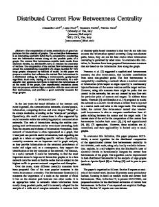
Fig. 1: Comparison of probability that EIC holds in ElasticNet and IC holds in LASSO in various number of random walks in the first dataset has used LASSO in its model. Moreover, in the theoretical proof of [5], they required that the graph is highly connected which may not be true in all of the real networks. Choosing

√ λ = M log M , k = 8 as sparsity, and N = 273 as the number of links in the first dataset, by increasing M such that M → ∞, Fig.1 shows that in CSCD model model consistency holds with higher probability. The rest of this section shows the evaluation of F-Score in our model in various settings. Fig. 2 illustrates an improvement of the F-Score performance of the CSCD model by an average of 5% (Dataset 1) and 10% (Dataset 2) for the various number of random walks compared to the Compressive Sensing over Graphs method (CS-over-Graph) presented in [5]. The number of random walks changes from 10% to 90% of the total network links. Although, we have evaluated F-Score for various random walk steps, the results were similar to those shown in Fig. 2. Clearly, for lower number of random walks, we have lower number of measurements, and thus less samples. Since the proposed model simultaneously employs the prior knowledge based on the link betweenness centrality, it performs better than CS-over-Graphs model [5] where only the sparsity information (kxk0 ) is used. However, as the number of random walks grows, our F-Score gets closer to CS-over-Graphs’. Because at higher number of random walk the prior knowledge becomes less significant. As

random walks when F-Score equals to 50%. The number of random walks in CSCD is decreased by an average of 16% in the first dataset and 15% in the second one compared to CSover-Graphs. We also compare the F-Score of our model with

Fig. 4: Sparsity versus various number of random walks in two datasets the algorithm that is used only Betweenness Centrality (BC) measurement for congestion detection (BC algorithm) as employed in [8], [9], and [10]. The result is illustrated in Fig. 5. Since betweenness centrality is independent from the number

(a)

(b)

Fig. 2: F-Score versus random walk number in two datasets illustrated in Fig. 3, we have also evaluated the F-Score of CSCD in terms of sparsity of the congested links in the network (kxk0 ). The F-Score of the CSCD model is improved by an average of 11% in the first dataset, and 9% in the second one compared to CS-over-Graphs model. In Fig. 4, we

Fig. 5: Comparison of our model with BC algorithm in terms of (a) the required number of random walks (b) sparsity of random walks, it remains constant in Fig. 5(a). As shown in Fig. 5, CSCD outperformed the algorithms based on mere betweenness centrality, by an average of 12% on F-Score for different sparsities and 69% on F-Score for various random walk numbers.

6. CONCLUSION

Fig. 3: F-Score versus sparsity in two datasets have measured the required number of random walks in terms of the sparsity of the congested links in the network (kxk0 ). Considering the sparsity varies from 5% to 30% of the network links, we have calculated the least required number of

In this paper, we introduced a new objective function based on the concepts of compressive sensing in a network tomography application. We used the link betweenness prior knowledge in our objective function which results in a decrease on the required number of measurements for detecting the network congested links. Based on extensive simulation results, we verified significant improvement in accuracy of detecting the network congested links in two real datasets.

7. REFERENCES [1] A. Davenport, F. Duarte, C. Eldara, and G. Kutyniok, Introduction to Compressed Sensing, Compressed Sensing: Theory and Applications, Cambridge University Press, 2011. [2] Y. Huang and N. Feamster, “Practical issues with using network tomography for fault diagnosis,” ACM SIGCOMM 2008, August 2008, Seattle, WA, USA. [3] Y. Vardi, “Network tomography: Estimating sourcedestination traffic intensities from link data,” Journal of the American Statistical Association, 1996. [4] R. Gaeta, M. Grangetto, and M. Sereno, “Local access to sparse and large global information in p2p networks: a case for compressive sensing,” IEEE Tenth International Conference on Peer-to-Peer Computing (P2P), August 2010, Delft, Netherlands. [5] W. Xu, E. Mallada, and A. Tang, “Compressive sensing over graphs,” Proc. IEEE INFOCOM, April 2011, Shanghai,China. [6] J. Jia and B. Yu, “On model selection consistency of the elastic net when p ¿¿ n,” Statistica Sinica., vol. 20, pp. 595–611, May 2010. [7] M. Cheraghchi, A. Karbasi, S. Mohajer, and V. Saligrama, “Graph-constrained group testing,” IEEE Transactions on Information Theory, vol. 58, no. 1, pp. 248–262, Jan. 2012. [8] P. Holme, “Congestion and centrality in traffic flow on complex networks,” Journal of Advanced Complex Systems, vol. 6, no. 2, pp. 163–176, 2003. [9] A. Leon-Garcia A. Tizghadam, “Betweenness centrality and resistance distance in communication networks,” IEEE Network, vol. 24, no. 6, pp. 10–16, 2010. [10] B. K. Singh and N. Gupte, “Congestion and decongestion in a communication network,” Physical Review E, vol. 71, no. 5, 2005. [11] R. Baraniuk, “Compressive sensing,” IEEE Signal Processing magazine, vol. 24, no. 4, pp. 118–120, 2007. [12] S. Ji, Y. Xue, and L. Carin, “Bayesian compressive sensing,” IEEE Transaction on Signal Processing, vol. 56, no. 6, pp. 2346–2356, 2008. [13] D. Baron, S. Sarvotham, and R. G. Baraniuk, “Bayesian compressive sensing via belief propagation,” IEEE Transactions on Signal Processing, vol. 58, no. 1, pp. 269–280, 2010.

[14] S. Babacan, R. Molina, and A. Katsaggelos, “Bayesian compressive sensing using laplace priors,” IEEE Transactions on Image Processing, vol. 19, no. 1, pp. 53–64, 2010. [15] M. Barthelemy, “Betweenness centrality in large complex networks,” The European Physical Journal B (Condensed Matter and Complex Systems), vol. 38, pp. 163– 168, 2004. [16] A. Gronlund and P. Holme, “A network-based threshold model for the spreading of fads in society and markets,” Advances Complex Systems Journal, vol. 8, no. 2, pp. 261–273, 2003.