Fast exact computation of betweenness centrality in social networks Miriam Baglioni∗ , Filippo Geraci∗ , Marco Pellegrini∗ and Ernesto Lastres† - CNR, Via Moruzzi 1, Pisa 56124, Italy. Tel +39-050-3152410, {m.baglioni, f.geraci, m.pellegrini}@iit.cnr.it † Sistemi Territoriali, via di Lupo Parra Sud 144 San Prospero 56023 (PI), Italy. Tel. +39-050-768711,
[email protected] ∗ IIT
Abstract—Social networks have demonstrated in the last few years to be a powerful and flexible concept useful to represent and analyze data emerging form social interactions and social activities. The study of these networks can thus provide a deeper understanding of many emergent global phenomena. The amount of data available in the form of social networks data is growing by the day, and this poses many computational challenging problems for their analysis. In fact many analysis tools suitable to analyze small to medium sized networks are inefficient for large social networks. The computation of the betweenness centrality index is a well established method for network data analysis and it is also important as subroutine in more advanced algorithms, such as the Girvan-Newman method for graph partitioning. In this paper we present a new approach for the computation of the betweenness centrality, which speeds up considerably Brandes’ algorithm (the current state of the art) in the context of social networks. Our approach exploits the natural sparsity of the data to algebraically (and efficiently) determine the betweenness of those nodes forming trees (tree-nodes) in the social network. Moreover, for the residual network, which is often of much smaller size, we modify directly the Brandes’ algorithm so that we can remove the nodes already processed and perform the computation of the shortest paths only for the residual nodes. Tests conducted on a sample of publicly available large networks from the Stanford repository show that improvements of a factor ranging between 2 and 5 are possible on several such graphs, when the sparsity, measured by the ratio of treenodes to the total number of nodes, is in a medium range (30% to 50%). For some large networks from the Stanford repository and for a sample of social networks provided by Sistemi Territoriali with high sparsity (80% and above) tests show that our algorithm consistently runs between one and two orders of magnitude faster than the current state of the art exact algorithm. Keywords-Betweenness centrality, social network analysis
I. I NTRODUCTION Social networks have demonstrated in the last few years to be a powerful and flexible concept useful to represent and analyze data emerging form social interactions and social activities. The study of these networks can thus provide a deeper understanding of many emergent social global phenomena. Moreover such analytic tools and concepts have been successfully adopted in a vast range of applications including communications, marketing and bioinformatics. According to the standard paradigm of social networks, to each agent/item is associated a node of the network and the edges between pairs of nodes represent the relationship between them. Social networks are naturally represented as
graphs, consequently graph theory and efficient graph algorithms plays an important role in social network analysis. Among the analytic tools, centrality indices are often used to score (and rank) the nodes (or the edges) of the network to reflect their centrality position. The intuitive idea behind this class of indices is that a more central node is likely to be involved in many processes of the network, thus its importance increases. Depending on what we mean with the word “important”, different definitions of centrality are possible [1]. For example degree centrality highlights nodes with a higher number of connections, closeness centrality highlights nodes easily reachable from other nodes, and eigenvector centrality highlights nodes connected with authoritative nodes. A complete compendium of many centrality definitions, problems and measures can be found in [2]. Vertex betweenness [3], [4] is one of the most broadly used centrality indices. The (vertex) betweenness of a vertex v is defined as the sum, for each pair of nodes (s, t) in the network, of the ratio between the number of shortest (aka geodesic) paths from s to t passing through v and the total number of shortest paths from s to t. The main assumption of this index is that the information flows in the network following shortest paths. Despite the fact that this assumption could be considered restrictive, betweenness finds a vast range of applications (e.g. in computing lethality for biological networks [5] and in bibliometry [6]). A very similar concept of edge betweenness is defined in [3] where for an edge e, the sum is computed for each pair of nodes (s, t) of the ratio among the number of shortest paths from s to t through the edge e over the number of all the shortest paths from s to t. Edge betweenness has a prominent application as a subroutine in the algorithm of Newman and Girvan [7] for community detection of complex networks. In this paper, for sake of clarity, we discuss only the problem of computing efficiently vertex betweenness, however with minor modifications our approach applies to edge betweenness as well (see [8]). The computation of the betweenness centrality index is demanding because, for a given node v, all the shortest paths between each couple of nodes passing through v have to be counted (even if it is not necessary to explicitly enumerate them). This means that, in general, for fairly large networks the computation of this index based on a direct application of its definition becomes impractical, having complexity O(n3 ), for a graph with n nodes. Since the last decade the number and size of social networks have
been consistently increasing over time, efficient algorithms have emerged to cope with this trend. The fastest exact algorithm to date is due to Brandes [9]. It requires O(n + m) space and O(nm) time where n is the number of nodes and m the number of edges in the graph. For sparse graphs, where m = O(n), Brandes’ method is a huge improvement over the naive direct method, however it is still quadratic in n, regardless of any other special feature the input graph may have. In this paper we propose an evolution of the Brandes’ algorithm which exploits some widespread topological characteristic of social networks to speed up the computation of the betweenness centrality index. We show that for nodes in the graph that belong to certain tree structures the beteenness value can be computed by a straightforward counting argument. The advantage of our approach is twofold: on the one hand we do not need to count shortest paths for the subset of network nodes that have the required tree-structure, and, on the other hand, for the residual nodes we compute the shortest paths only between nodes belonging to the residual of the original graph, thus more efficiently. Our algorithm performance strictly depends on the number of nodes for which we can algebraically derive the betweenness. Therefore it works well in practice for social networks since we observed that such tree structures are quite frequent in the context of social networks where the number of edges of the graph is of the same order of magnitude of the number of nodes. Note, however, that our algorithm still reduces to the Brandes’ algorithm in a strict worst case scenario. We tested our algorithm on a set of 18 social graphs of Sistemi Territoriali which is an ICT company with headquarters in Italy, specializing in Business Intelligence applications. These graphs coming from real applications are very large and very sparse, a property our algorithms exploits to gain in efficiency. Compared to Brandes’ method we can gain orders of magnitudes (between one and two) in terms of computation time. We tested our algorithm on a set of 16 social graphs from the Stanford Large Network Dataset Collection. We obtained marginal improvements on 7 cases, speed ups by a factor from 2 to 6 in 6 cases, and speedups by orders of magnitude in two cases. At the best of our knowledge this approach is novel. The paper is organized as follows. Section II gives a brief survey of related work, while section III gives key insights from Brandes’ methods. In section IV we describe our method in detail. In Section V we give the experimental results. II. R ELATED WORK Let G = (V, E) be the graph associated to a social network, we denote as: σst the number of shortest paths starting from the node s and ending in t, σst (v) the cardinality of the subset of geodesic paths from s to t passing through v. Betweenness centrality [4] measures, for a given vertex v, the fraction of all the possible shortest paths between
pairs of nodes which pass through v. Formally betweenness centrality B(v) is defined as: X σst (v) B(v) = σst s6=v6=t∈V
The practical application of centrality indices depends also on the scalability of the algorithm designed to compute them. Early exact algorithms have a complexity in the order of O(n3 ) [10], where n is the number of nodes. Thus the computation of betweenness by this direct approach becomes impractical for networks with just a few thousands of nodes. In 2001 Brandes [9] developed the asymptotically fastest exact algorithm to date, that exploits a recursive formula for computing partial betweenness indices efficiently. It requires O(n + m) space and O(nm) time where n is the number of nodes and m the number of edges in the graph. For sparse graphs, where m = O(n), Brandes’ method is a huge improvement over the naive direct method, allowing to tackle graphs with tens of thousands of nodes. Given the importance of the index, and the increasing size of networks to be analyzed, several strategies for scaling up the computation have been pursued. Algorithms for parallel models of computations have been developed (se e.g. [11] and [12]). A second strategy is to resort to approximations of the betweenness [13]. In [14] the authors describe an approximation algorithm based on adaptive sampling which reduces the number of shortest paths computations for vertices with high centrality. In [15] the authors present a framework that generalizes the Brandes’ approach to approximate betweenness. In [16] the authors propose a definition of betweenness which take into account paths up to a fixed length k. Another important complexity reduction strategy was presented in [17] where ego-networks are used to approximate betweenness. A ego-network is a graph composed by a node, called ego, and by all the nodes, alters, connected to the ego. Thus if two nodes are not directly connected, there is only a possible alternative path which passes through the ego node. The authors have empirically shown over random generated networks that the betweenness of a node v is strongly correlated to that of the ego network associated to v. In order to extend the use of betweenness centrality to a wider range of applications, many variants of this index were proposed in the literature. For example in [18] the betweenness definition is applied to dynamic graphs, while in [19] geodesic paths are replaced with random walks. In this paper we propose to use specific local structures abundant in many types of social graphs in order to speed up the exact computation of the betweenness index of each node by an adaptation of the exact algorithm due to Brandes. We have tested graphs with up to 500K nodes, which is a fair size for many applications. However in some applications (e.g. web graphs, facebook friendship graphs), we face much larger graphs in the regions of millions
of nodes. In this case approximating betweenness may be the strategy of choice. Our approach can be adapted to an approximation setting such as the one described by Geisberger et al. [15], where approximation is attained by (a) using a random subset of source nodes s for the BFS instead of every possible node, and (b) by adopting a modified weighted variant of the recursive equation (2). III. BACKGROUND In this section we give some key features of Brandes’ algorithm, since it gives a background to our approach. This method is based on an accumulation technique where the betweenness of a node can be computed as the sum of the contributions of all the shortest paths starting from each node of the graph taken in turns. Given three nodes s, t, v ∈ V , Brandes introduces the pair-dependency of s and t on v as the fraction of all the shortest paths from s to t through v over those from s to t: σst (v) δst (v) = σst The betweenness centrality of the node v is obtained as the sum of the pair-dependency of each pair of nodes on v. To eliminate the direct computation of all the sums, Brandes introduces the dependence of a vertex s on v as: X δs• (v) = δst (v) (1) t∈V
Thus the betweenness centrality B, of node v is given by summing contributions from all source nodes: X B(v) = δs• (v) s∈V
Observation 1. If a node v is a predecessor of w in a shortest path starting in s, then v is a predecessor also in any other shortest path starting from s and passing through w [9]. Arguing form the observation 1, equation 1 can be rewritten as a recursive formula: X σsv (1 + δs• (w)), (2) δs• (v) = σsw w:v∈Ps (w)
where Ps (w) is the set of direct predecessors of a certain node w in the shortest paths from s to w, encoded in a BFS rooted DAG form node s. IV. O UR A LGORITHM Our algorithm algebraically computes the betweenness of nodes belonging to trees in the network obtained by removing iteratively nodes of degree 1. Afterwards we apply a modification of Brandes’ algorithm [9] to compute the betweenness of the nodes in the residual graph. A first trivial observation is that nodes with a single neighbor can be only shortest paths endpoints, thus their betweenness is equal to zero. Thus we would like to remove
these nodes from the graph. However, these nodes by their presence influence the betweenness of their (unique) neighbors. In fact, such neighbor v works as a bridge to connect the node to the rest of the graph and all the shortest paths to (from) this node pass through that unique neighbor. Our procedure computes the betweenness of a node v as the sum of the contribution of all nodes for which v is their unique direct neighbors. Following this strategy, once the contribution of the nodes with degree 1 has been considered in the computation of the betweenness of their neighbors, they provide no more information, and can be virtually removed from the graph. The removal of the nodes with degree 1 from the graph, can cause that the degree of some other node becomes 1. Thus the previous considerations can be repeated on a new set of degree one nodes. When we iterate, however, we need also to record the number of nodes connected to each of the degree one nodes that were removed from the graph. This recursive procedure allows us to algebraically compute the betweenness of trees in the graph. A. Algorithm formalization and description We will assume the input G to be connected, in order to simplify the argument. If G is not connected, the argument can be repeated for each connected component separately. Let F be the set of nodes in G = (V, E) that can be removed by iteratively delete nodes of degree 1, and their adjacent edge. We call the nodes in F the tree-nodes. Let G0 = (V 0 , E 0 ) be the residual graph for the residuals set of node, with V 0 = V \ F . The set F induces a forest in G, moreover the root of each tree Ti of the forest is adjacent to a unique vertex in V 0 . Each node in F is a root to a sub-tree. Let RG (w, F ) be the set of of nodes of trees in F having w as their root-neighbor in G0 . The formula for the betweenness of node v ∈ V involves a summation over pairs of nodes s, t ∈ V . Thus we can split this summation into sub-summations involving different types of nodes, and provide different algorithms and formulae for each case. Tree-nodes. Let u be a node in F , and let v1 , .., vk be the children of u in the tree Tu , and let Tvi , for i = 1, ..k, be the subtrees rooted at vi . When s and t are in the same subtree Tvi , then there is only one shortest path connecting them completely in Tvi and this path does not contain u, thus the contribution to B(u) is null. When s is in some tree Tvi , and t is in the complement (V \{u})\Tvi , then each shortest path connecting them will contain u. Thus the contribution to the betweenness of u is given by the number of such pairs. We will compute such number of pairs incrementally interleaved with the computation of the set F by peeling away nodes of degree 1 from the graph. When at iteration j, we peel away node vi we have recursively computed the value of |Tvi |, and also for the node u the value |RG (u, Fj )| which is the sum of the sizes of trees Tvh , for h ∈ [1, ..k], i 6= k already peeled away in previous iterations. The number of
new pairs to be added to B(u) is: |Tvi | × (|(V \ {u}) \ Tvi | − |RG (u, Fj )|). This ensures that each pair (s,t) is counted only once. Finally observe that when both s and t are in V 0 no shortest path between them will contain u therefore their contribution to B(u) is zero. Since the roles of s and t are symmetrical in the formula we need to multiply the final result by 2 in order to cont all pairs (s, t) correctly. The pseudocode for this procedure is shown in Section IV-B. Residual graph nodes. Let u be a node in V 0 , we will see how to modify Brandes’ algorithm so that executing the modified version on the residual graph G0 (thus at a reduced computational cost), but actually computing the betweenness of the nodes in u ∈ V 0 relative to the initial graph G. Brandes algorithm’s inner loop works by computing from a fixed node s a BFS search DAG in the input graph, which is a rooted DAG (rooted at s), and by applying a structural induction from the sinks of the DAG towards the root as in formula (2). Subcase 1. If a node x ∈ V 0 has R(x, F ) 6= ∅ the tree formed by R(x, F ) and x would be part of the BFS DAG in G having its source in V 0 , however, since we run the algorithm on the reduced graph G0 , we need to account for the contribution of the trimmed trees to the structural recursive formula (2). The correction term for δs• (x) is equal to |RG (x, F )| since each shortest path from s to y ∈ RG (x, F ) must contain x. Thus we obtain the new formula: X σsu (1 + δs• (w) + |RG (w, F )|)) δs• (u) = σsw w:u∈Ps (w)
Note that in the development of the above formula R(s, F ) does not appear. Since no shortest path from s ∈ V 0 to any t ∈ R(s, F ) may include a node u ∈ V 0 , this subtree has zero contribution to δs• (u). Subcase 2. Consider now a node x ∈ R(s, F ) as source for the BFS. In the computation of δx• (u), for u ∈ V 0 each shortest path from x to t ∈ R(s, F ) cannot contain u thus gives zero contribution. For t ∈ V \ R(s, F ), such shortest path would contain a shortest path from s, thus we have δx• (u) = δs• (u) for all x ∈ R(s, F ). In order to account for these contributions to B(u) it suffices to multiply the contribution δs• by (1 + |R(s, F )|), obtaining: B(u) = B(u) + δs• (u) ∗ (1 + RG (s, F )). B. Algorithm pseudo-code In the following Algorithm 1 we show the pseudo-code for SPVB (Shortest-paths vertex betweenness) preprocessing, handling degree 1 nodes. For simplicity we assume G to be connected. For a disconnected graph G, the algorithm should be applied to each connected component separately. For a node v of degree 1 at a certain stage of the iteration, the vector p records the number of nodes in a subtree rooted at v
(excluding the root). For any other node u, vector p records the sum of the sizes of subtrees rooted at children of that node that have been deleted in previous iterations. SPVB: Data: undirected unweighted graph G=(V,E) Result: the graph’s node betweenness B[v] for all v∈V B[v] = 0, v ∈ V ; p[v] = 0, v ∈ V ; i = 0; Gi = G; deg1 = {v ∈ V i |deg(v) = 1}; repeat v ← deg1 ; u ∈ V i .(v, u) ∈ E i ; B[u] = B[u] + 2(n − p[v] − p[u] − 2)(p[v] + 1); remove v from deg1 ; p[u] = p[u] + p[v] + 1; i + +; V i = V i−1 \{v} E i = E i−1 \{(v, u)} if deg(u) = 1 then u → deg1 ; /* deg(u) is computed on the new graph Gi */ until deg1 = ∅ ; if |V i | > 1 then Brandes modified(Gi , p, B) end Algorithm 1: Shortest-paths vertex betweenness The modification of Brandes’ algorithm does not change its asymptotic complexity, which however must be evaluated on the residual graph with n0 = |V | − |F | nodes and m0 = |E| − |F | edges, thus with a time complexity O(n0 m0 ). The complexity of the first part of SPVB is constant for each node in F , except for the operations needed to dynamically modify the graph Gi and maintain the set of degree-1 nodes. With standard dynamic dictionary data structure we have an overhead of O(log n) for each update operation. V. E XPERIMENTS In order to evaluate the performance of our algorithm we run a set of experiments using both a collection of 18 graphs provided by Sistemi Territoriali (SisTer), which is an Italian ICT company involved in the field of data analysis for Business intelligence and a collection of graphs downloaded from the Stanford Large Network Dataset Collection1 . Since both our algorithm and Brandes’ compute the exact value of betweenness, we tested the correctness of the implementation by comparing the two output vectors. Here we report only on the the running time of the two algorithms. For our experiments we used a standard PC endowed with a 2.5 GHz Intel Core 2, 8Gb of RAM and Linux 2.6.37 operating system. The two algorithms were implemented in Java. In order to avoid possible biases in the running time evaluation due to the particular CPU architecture, we 1 http://snap.stanford.edu/data/
Brandes modified: Data: directed graph G = (V, E), for each v: the number of tree-nodes connected to v: p[v], the partial betweenness computed for v: B[v] Result: the graph’s node betweenness B[v] for s ∈ V do S = empty stack; P[w]= empty list,w ∈ V ; σ[t] = 0, t ∈ V ;σ[s] = 1; d[t] = −1, t ∈ V i ; d[s] =0; Q= empty queue; enqueue s → Q; while Q not empty do dequeue v ← Q; push v → S; forall neighbor w of v do // w found for the first time? if d[w] < 0 then enqueue w → Q; d[w]=d[v] + 1; end // shortest path to w via v? if d[w] = d[v] + 1 then σ[w] = σ[w] + σ[v]; append v → P [w]; end end end δ[v] = 0, v ∈ V ; // S returns vertices in order of non-increasing distance from s while S not empty do pop w← S; for v ∈ P[w] do σ[v] δ[v] = δ[v] + σ[w] (δ[w] + p[w] + 1); end if w 6= s then B[w] = B[w] + δ[w] × (p[s] + 1) end end end Algorithm 2: Modified Brandes’ algorithm
decided to implement the algorithm as a mono-processor sequential program. SisTer Collection. In table I we report the graph id, the number of nodes and edges in the SisTer collection and the percentage of tree-nodes in each graph. Note that a very large percentage of the nodes can be dealt with algebraically by our algorithm and the residual graph, on which we ran a modified Brandes’, is quite small relative to the original size. Figure 1 compares the running time of our and Brandes’
Graph ID G1 G2 G3 G4 G5 G6 G7 G8 G9 G10 G11 G12 G13 G14 G15 G16 G17 G18
Node # 233,377 14,991 15,044 16,723 16,732 169,059 16,968 3,214 3,507 3,507 3,519 44,550 46,331 47,784 5,023 52,143 8,856 506,900
Edge # 238,741 14,990 15,101 16,760 16,769 169,080 17,026 3,423 3,620 3,620 3,632 46,519 46,331 48,461 5,049 53,603 10,087 587,529
Tree nodes (%) 86 % 99 % 85 % 84 % 84 % 99 % 84 % 95 % 96 % 96 % 96 % 77 % 99 % 84 % 93 % 85 % 89 % 80 %
Table I S IS T ER C OLLECTION . F OR EACH GRAPH IT IS LISTED THE NUMBER OF NODES , THE NUMBER OF EDGES , AND THE PERCENTAGE OF TREE - NODES . T HE GRAPHS NEED NOT BE CONNECTED .
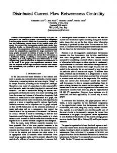
Figure 1. A comparison of the running time of our algorithm (left) and Brandes’ (right) on 18 sparse large graphs. The ordinate axis report running time in seconds and is in logarithmic scale. Data for Brandes on graph 18 is missing due to time-out
algorithms. On the x-axis we report the graph id, while on the y-axis we report in logarithmic scale the running time expressed in seconds. From figure 1 it is possible to observe that our algorithm is always more than one order of magnitude faster than the procedure of Brandes, sometimes even two orders of magnitude faster. For graph G1, with 233,377 nodes for example, we were able to finish the computation within one hour while Brandes’ needs approximately two days. For graph G6, with 169,059 nodes, we could complete in about 1 minute, compared to two days for Brandes. A notable result is shown also for graph
Graph name ca-GrQc as20000102 ca-HepTh ca-HepPh ca-AstroPh ca-CondMat as-caida20071112 cit-HepTh cit-HepPh p2p-Gnutella31 soc-epinion1 soc-sign-Slashdot090221 soc-Slashdot0922 soc-sign-epinions Email-EuAll web-NotreDame
Node # 5,242 6,474 9,877 12,008 18,772 23,133 26,389 27,770 34,546 62,586 75,879 82,144 82,168 131,828 265,214 325,729
Edge # 28,980 13,233 51,971 237,010 396,160 186,936 106,762 352,807 421,578 147,892 508,837 549,202 948,464 841,372 420,045 1,497,134
Tree nodes (%) 21% 36% 20% 11% 6% 9% 38% 5% 4% 46% 51% 36% 2% 51% 80% 51%
Table II S ELECTED GRAPHS FROM THE S TANFORD C OLLECTION . F OR EACH GRAPH IT IS LISTED THE NUMBER OF NODES , THE NUMBER OF EDGES , AND THE PERCENTAGE OF TREE - NODES , WHICH IS THE MOST IMPORTANT PARAMETER AFFECTING THE TIME PERFORMANCE .
G18 which is our biggest in this collection. In this case our algorithm required approximately 2,4 days to finish while Brandes’ could not terminate in one month (data not shown). Stanford Collection. We have selected a subset of graphs from the Stanford collection, using the following criteria. First the graphs have been ranked by number of nodes and we have selected representative graphs from as many categories as possible (Social networks, Communication Networks, Citation networks, Collaboration networks, Web graphs, Internet peer-to-peer networks, and Autonomous systems graphs). We have excluded graphs that because of their size would take more than one week of computing time. In Table (II) we have listed these graphs, their size in number of nodes and edges, and the percentage of tree-nodes, which is the most important parameter influencing the performance of our method. Each input graph was considered undirected. We decided a cut-off time of seven days. In order to measure the convergence of the two methods we collected also the partial output of the two algorithms every 24 hours of execution. In table III the running time, expressed in seconds, of the two methods is shown, and the speed up factor. As it is expected the speed up factor is strongly correlated to the fraction of the tree-nodes in the graph. We notice a speed-up factor ranging from 2 to almost 6 when the ratio of tree-nodes to the total number of nodes is in the range 30% to 50%. Two large test graphs are quite noticeable. Graph EmailEuAll has a percentage of 80% of tree-nodes which is a value closer to those found in the SisTer collection, thus the speed up measured is at least 27 (since we stopped Brandes’ after one week). That value is between one and two orders of magnitude, consistently with those measured in the SisTer collection. For the web-NotreDame graph, which is the largest graph
Graph name ca-GrQc as20000102 ca-HepTh ca-HepPh ca-AstroPh ca-CondMat as-caida20071112 cit-HepTh cit-HepTh p2p-Gnutella31 soc-Epinion1 soc-sign-Slashdot090221 soc-Slashdot0902 soc-sign-epinions Email-EuAll web-NotreDame
Node # 5,242 6,474 9,877 12,008 18,772 23,133 26,389 27,770 34,546 62,586 75,879 82,140 82,168 131,828 265,214 325,729
Brandes (s) 35 s 141 s 230 s 703 s 2,703 s 3,288 s 6,740 s 8,875 s 16,765 s 74,096 s 145,350 s 199,773 s 199,544 s 564,343s > 7 days -
Ours (s) 24 s 54 s 148 s 563 s 2,447 s 2,718 s 2,014 s 8,227 s 15,636 s 15,573 s 25,771 s 64,905 s 190,536 s 96,738 s 22,057 s ≈ 9 days
Ratio 1.45 2.65 1.55 1.24 1.10 1.21 3.34 1.07 1.07 4.76 5.64 3.07 1.04 5.83 > 27 ≈8
Table III RUNNING TIME ( IN SECONDS ) OF THE TWO METHODS OVER SELECTED S TANFORD C OLLECTION GRAPHS , AND THEIR RATIO ( SPEED UP FACTOR ).
in our sample of the Stanford collection, we estimate the convergence properties of the two algorithms as follows. Our algorithm has been run to completion (in about 9 days) in order to have the exact target solution vector. Also at fixed intervals each day we recorded the intermediate values of the betweenness vectors for both algorithms. For each vertex we compute the ratio of the intermediate value over the target value (setting 0/0 to value 1), and then we average over all the vertices. This measure is strongly biased by the fact that for leaves (nodes with degree 1) both Brandes and our algorithm assign at initialization the correct value 0, thus in this case precision is attained by default. To avoid this bias we repeat the measurement by averaging only over those nodes with final value of betweenness greater than zero (see Figure 2). From figure 2 we can appreciate that the average convergence rate is almost linear in both case, but the curve for our algorithm has a much higher slope. After 7 days our algorithm reached about 75% of the target, against 10% of Brandes’, by a linear extrapolation we can thus predict a speed up factor of about 8.
VI. C ONCLUSIONS AND ACKNOWLEDGMENTS Brandes’ algorithm for computing betweenness centrality in a graph is a key breakthrough beyond the naive cubic method that computes explicitly the shortest paths in a graph. However, it is not able to exploit possible additional locally sparse features of the input graph to speed up further the computation on large graphs. In this work we show that combining exact algebraic determination of betweenness centrality for some tree-like sub-graphs of the input graph, with a modified Brands’ procedure on the residual graph we can gain orders of magnitudes (between one and two) in terms of computation time for very sparse graphs, and a good factor from 2 to 5, in moderately sparse graphs. At the
[6] L. Leydesdorff, “Betweenness centrality as an indicator of the interdisciplinarity of scientific journals,” Journal of the American Society for Information Science and Technology, vol. 58, pp. 1303–1309, July 2007. [7] M. Girvan and M. E. J. Newman, “Community structure in social and biological networks,” PNAS, vol. 99, no. 12, pp. 7821–7826, 2002. [8] U. Brandes, “On variants of shortest-path betweenness centrality and their generic computation,” Social Networks, vol. 30, no. 2, pp. 136 – 145, 2008. [9] ——, “A faster algorithm for betweenness centrality,” Journal of Mathematical Sociology, vol. 25, no. 2, pp. 163–177, 2001. Figure 2. Evolution in time of the average (over the vertices) ratio of the partial betweenness values over the final betweenness value. In the averaging leaves are excluded.
best of our knowledge this approach is novel. In our test set we did not find a significant number of tree-nodes only in author collaboration graphs, and citation graphs, while for the other categories in this test set we did find a significant number of tree-nodes. We thus conjecture that this feature is common enough in a range of social networks so to make the application of our method an interesting option when exact betweenness is to be computed. As future work we plan to explore further this approach by expoloring the role of articulation points and determining other classes of subgraphs (besides trees) in which we can gain by the direct algebraic determination of the betweenness. Moreover the impact of our approach combined with approximation schemes will be investigated. This research is partially supported by the project BINet “Nuova Piattaforma di Business Intelligence Basata sulle Reti Sociali” funded by Regione Toscana POR CReO 2007-2013 Programme. R EFERENCES [1] D. Koschatzki, K. Lehmann, L. Peeters, S. Richter, D. Tenfelde-Podehl, and O. Zlotowski, “Centrality indices,” in Network Analysis, ser. LNCS, U. Brandes and T. Erlebach, Eds. Springer Verlag, 2005, vol. 3418, pp. 16–61. [2] S. P. Borgatti, “Centrality and network flow,” Social Networks, vol. 27, no. 1, pp. 55 – 71, 2005. [3] J. M. Anthonisse, “The rush in a directed graph,” Stichting Mathematisch Centrum, 2e Boerhaavestraat 49 Amsterdam, Tech. Rep. Tech. Rep. BN 9/71, October 1971. [4] L. C. Freeman, “A Set of Measures of Centrality Based on Betweenness,” Sociometry, vol. 40, no. 1, pp. 35–41, Mar. 1977. [5] A. Del Sol, H. Fujihashi, and P. O’Meara, “Topology of small-world networks of protein–protein complex structures,” Bioinformatics, vol. 21, pp. 1311–1315, April 2005.
[10] R. Jacob, D. Koschtzki, K. Lehmann, L. Peeters, and D. Tenfelde-Podehl, “Algorithms for centrality indices,” in Network Analysis, ser. LNCS, U. Brandes and T. Erlebach, Eds. Springer Verlag, 2005, vol. 3418, pp. 62–82. [11] K. Madduri, D. Ediger, K. Jiang, D. A. Bader, and D. Chavarria-Miranda, “A faster parallel algorithm and efficient multithreaded implementations for evaluating betweenness centrality on massive datasets,” Parallel and Distributed Processing Symposium, International, vol. 0, pp. 1–8, 2009. [12] D. Bader and K. Madduri, “Parallel algorithms for evaluating centrality indices in real-world networks,” in ICPP 2006, aug. 2006, pp. 539 –550. [13] U. Brandes and C. Pich, “Centrality estimation in large networks,” I. J. Bifurcation and Chaos, vol. 17, no. 7, pp. 2303–2318, 2007. [14] D. Bader, S. Kintali, K. Madduri, and M. Mihail, “Approximating betweenness centrality,” in Algorithms and Models for the Web-Graph, ser. LNCS, A. Bonato and F. Chung, Eds. Springer Verlag, 2007, vol. 4863, pp. 124–137. [15] R. Geisberger, P. Sanders, and D. Schultes, “Better approximation of betweenness centrality,” in ALENEX, 2008, pp. 90–100. [16] S. White and P. Smyth, “Algorithms for estimating relative importance in networks,” in Proceedings of the ninth ACM SIGKDD. New York, NY, USA: ACM, 2003, pp. 266–275. [17] M. Everett and S. P. Borgatti, “Ego network betweenness,” Social Networks, vol. 27, no. 1, pp. 31 – 38, 2005. [18] T. Carpenter, G. Karakosta, and D. Shallcross, “Practical issues and algorithms for analyzing terrorist networks,” 2002, invited paper at WMC 2002. [19] M. J. Newman, “A measure of betweenness centrality based on random walks,” Social Networks, vol. 27, no. 1, pp. 39 – 54, 2005.