Incorporating Body Dynamics into the Sensor-Based Motion Planning. Paradigm. .... nite length, such that a straight line will cross it only in a nite number of ...
Incorporating Body Dynamics into the Sensor-Based Motion Planning Paradigm. The Maximum Turn Strategy.� Vladimir J. Lumelsky and Andrei M. Shkel University of Wisconsin-Madison Madison, Wisconsin 53706, USA Abstract|The existing approaches to sensor-based motion planning tend to deal solely with kinematic and geometric issues, and ignore the system dynamics. This work attempts to incorporate body dynamics into the paradigm of sensor-based motion planning. We consider the case of a mass point robot operating in a planar environment with unknown arbitrary stationary obstacles. Given the constraints on the robot's dynamics, sensing, and control means, conditions are formulated for generating trajectories which guarantee convergence and the robot's safety at all times. The approach calls for continuous computation and is fast enough for real time implementation. The robot plans its motion based on its velocity, control means, and sensing information about the surrounding obstacles, and such that in case of a sudden potential collision it can always resort to a safe emergency stopping path. Simulated examples demonstrate the algorithm's performance.
because of the robot's mass and velocity. A step reasonable from the standpoint of reaching the target position { for example, a sharp turn { may not be physically realizable because of the robot's inertia (as at point P , Fig. 1). The existing strategies for sensor-based planning usually deal solely with the system kinematics and geometry and ignore its dynamic properties. Most approaches to automatic motion planning adhere to one of two paradigms which di�er in the assumptions about the information available for planning. In the rst paradigm, called motion planning with complete information (or the Piano Mover's problem), perfect information about the robot and the obstacles is assumed, their shapes are presented algebraically, and the motion planning is a onetime o�-line operation (see, e.g., [1, 2]). Dynamics and control constraints can be incorporated into this model as well [3], for example by introducing a two-stage planning process, time-optimal trajectories [4, 5]. This paper is concerned with the second paradigm, called motion planning with incomplete information, or sensorbased motion planning. In this model, the objects in the environment can be of arbitrary shape, and the input information is typically of local character, such as from a range nder or a vision sensor [6]. By making use of the notion of sensor feedback, this paradigm naturally ts the methodology of control theory, in particular techniques for continuous dynamic on-line processes. Techniques that ignore the dynamic issues can be called kinematic, as opposed to the dynamic techniques which take into account the body dynamics. The existing kinematic techniques can be divided into two groups { those for holonomic systems and for nonholonomic systems [7]. A number of kinematic strategies for holonomic systems originate in maze-searching algorithms [6, 8]; when applicable, they are usually fast, can be used for real time control, and guarantee convergence; the obstacles can be of arbitrary shape. Below we make of use of such algorithms. To design a provably-correct dynamic algorithm for sensor-based motion planning, one needs a single control mechanism { separating it into stages is likely to destroy
I. Introduction
This work studies the e�ect of body dynamics on robot sensor-based motion planning, with the goal of designing provably correct algorithms for motion planning in an uncertain environment. We consider a mobile robot operating in a planar environment lled with unknown arbitrary stationary obstacles. Planning is done in small steps (say, 30 or 50 times per second), resulting in a continuous motion. The robot is equipped with sensors, such as vision or range nders, which allow it to detect and measure distances to surrounding objects within its sensing range (\radius of vision"). This range covers a number of robot steps { say, 5 or 50 or 1000 { so that normally the robot would see an obstacle far enough to plan a collision-avoiding maneuver. Besides the usual planning problems of \where to go" and how to provide convergence in view of incomplete information, an additional, dynamic component of planning appears � This work is supported in part by the US Sea Grant R/NI-20 and DOE (Sandia Labs) Grant 18-4379C. 1
2
convergence. Convergence has two faces { globally it's a guarantee of nding a path to the target if one exists, and locally it's a guarantee of collision avoidance in view of the robot's inertia. The former can be borrowed from kinematic algorithms; the latter requires an explicit consideration of dynamics. Imagine a runner who starts turning the corner and suddenly sees a heavy large object right on the intended path. Clearly, some quick replanning will take place, almost simultaneous with further sensing and motion execution. The runner's velocity may temporarily decrease and the path will smoothly divert from the object. Or, he might \brake" to a halt along the initial path, and then start a detour path. Note that sensing, planning, and movement are taking place simultaneously and continuously. Unless a right relationship is maintained between the velocity at the time of noticing the object, the distance to it, and the runner's mass, collision may occur. For a bigger mass, for example, better (further) sensing is needed to maintain the same velocity. Also, if obstacles can appear at any time and distance, and if higher velocities are essential, the control algorithm must provide an \insurance" option of a safe stopping at all times. Although the robot has complete knowledge of the obstacles within its sensing range, because of the computational and convergence problems it would be di�cult to address the problem as a sequence of smaller problems with complete information. Our step-by-step calculation algorithm thus operates as a single procedure which (a) places each step on a globally converging collision-free path, while (b) satisfying the robot dynamics constraints. Assume that the sensing range (\radius of vision") is rv , Fig. 1. The general strategy is as follows: at the moment (step) i, the kinematic algorithm identi es an intermediate target point, Ti , which lies on a convergent path and, for local path optimization, is far enough from the robot { normally at the boundary of the sensing range. Then, a step is made in the direction of Ti , and the process repeats. Because of the dynamics, this step toward Ti may not be possible and needs to be modi ed. As mentioned above, sometimes stopping may be the only way to avoid collision, and an assurance is required that at any moment the robot could execute a last resort stopping path if needed. Since no information is available beyond the sensing range, the whole stopping path, as computed at a given moment, must lie within that sensing area. Further, since part of the sensing range may be invisible because of obstacles, the stopping path must lie in the visible part of the sensing range. Similarly, if the intermediate target Ti lies on the boundary of the sensing range, the robot needs a guarantee of stopping at Ti , even if at the moment it does not intend to do so. Thus, each step is to be planned as the rst step of a trajectory which, given the initial position, velocity and control constraints, would bring the robot to a
Robot’s path
T
Q
P
L
C Obstacle H
M-line
S rv
Fig. 1. Example of performance of the (kinematic) VisBug algorithm.
halt at Ti . In case of a curved path segment, the control system will attempt a reasonably fast convergence to Ti by trying to align the direction of the robot's motion with the direction toward Ti as soon as possible. That is, if the angle between the current velocity vector and the direction toward Ti is larger than the maximum turn the robot can make in one step, the robot will keep turning in the maximum way possible until the directions align (hence the name Maximum Turn Strategy). Once a step is physically executed, new sensing information appears and the process repeats. The procedure also covers a special case where the intermediate target goes out of the robot's sight because of the robot's inertia or because of occluding obstacles. The model assumed is introduced in Section II, followed by the sketch of the suggested approach in Sec. III. Analysis of the system dynamics appears in Sec. IV; the algorithm and its convergence properties are discussed in Sec. V, and simulated examples of the algorithm performance in Sec. VI. Some details and proofs are omitted due to space limitations. II. The model
The environment (the scene) is a plane; it may include a locally nite number of static obstacles. Each obstacle is bounded by a simple closed curve of arbitrary shape and of nite length, such that a straight line will cross it only in a nite number of points. Obstacles do not touch each other (if they do, they are considered one obstacle). Note that the model does not require the number of obstacles be nite. The robot is a mass point, of mass m. Its sensors allow it, at its current location Ci , to detect any obstacles and the distance to them within its sensing range { a disc of radius rv (\radius of vision") centered at Ci . At moment ti , the robot's input information includes its current velocity vector
3
Vi , coordinates of Ci and of the target point T it is trying VisBug algorithm [6], which is based on these two steps (as
to reach, and perhaps of few other points of interest, such as an intermediate target. The task is to move from point S (start) in the scene to point T (target), see Fig. 1. The robot's means for motion control are two components of the acceleration vector u = mf = (p; q), where m is the robot's mass, and f is the force applied. By taking, without loss of generality, mass m = 1, we can refer to the components p and q as if they represent control forces, each within its xed range jpj � pmax, jqj � qmax ; pmax; qmax > 0. Force p controls the forward (or backward when braking) motion; its positive direction coincides with the robot's velocity vector V. Force q is perpendicular to p forming a right pair of vectors, and is equivalent to the steering control (rotation of vector V), Fig. 2. The M-line (Main line) is the straight line connecting points S and T , and is the robot's desired path. When, while moving along the M-line, the robot senses on its way an obstacle, this point on the obstacle boundary is called a hit point, H . The corresponding M-line point \on the other side" of the obstacle is a leave point, L. The control of robot motion is done in steps i = 0; 1; 2; ::: . Each step i takes the same time � = ti+1 ? ti = const; its length thus depends on the robot's velocity within the step. Steps i and i + 1 start at times ti and ti+1 , respectively; C0 = S . We de ne two coordinate systems (follow Fig. 2): (i) The world coordinate frame, (x; y), xed at point S . (ii) The path coordinate frame, (t; n), which describes the motion of the mass point at any moment � 2 [ti ; ti+1 ) within the step i. Its origin is attached to the robot; axis t is aligned with the current velocity vector V, axis n is normal to t. Together with axis b, which is a cross product b = t � n, the triple (t; n; b) forms the Frenet trihedron, with the plane of t and n being the osculating plane. III. The approach
The algorithm will be executed at each step of the robot's path, as a single operation. We take the convergence mechanism of a kinematic sensor-based motion planning algorithm, and add to it controls for handling dynamics. At any moment ti the robot will maintain an intermediate target point Ti within its sensing range, usually on an obstacle boundary or on the M-line. At its current position Ci , the robot will plan and execute its next step in the direction Ti , then, at Ci+1 analyze new sensory information and perhaps de ne a new intermediate target Ti+1 , and so on. At times, the current Ti may go out of the robot's sight because of its inertia or due to occluding obstacles. In such cases the robot will be designate temporary intermediate targets and use them until it can see point Ti again. In principle, any maze-searching algorithm can be utilized for the kinematic part, so long as it allows an extension to distant sensing. For the sake of speci city, we use here the
before, S and T are starting and target positions, rv the radius of the sensing range, Fig. 1): (1) Walk from S toward T along the M-line until, at some point C , detect an obstacle crossing the M-line, say at point H ; go to Step 2. (2) Using sensors, de ne the farthest visible intermediate target Ti on the obstacle boundary; make a step toward Ti ; iterate Step 2 until detect M-line; go to Step 1. In Fig. 1, note that while trying to pass the obstacle from the left, at point P the robot will make a sharp turn. Safety considerations due to dynamics appear in a number of ways. Since no information about the obstacles is available beyond distance rv from the robot, guaranteeing collisionfree motion means assuring at any moment at least one \last resort" path that would bring the robot to a halt within the radius rv if needed. If this rule is violated, at the next step new obstacles may appear in the sensing range, such that collision will become imminent no matter what control is used. This dictates a certain relation between the velocity V, mass m, and controls u = (p; q): if the robot moves with the maximum velocity, the stop point of the stopping p path must be no further that at distance rv from C , V = 2prv . In Fig. 1, when approaching point P , the robot will designate it as its next intermediate target Ti . For awhile Ti will stay at P because no other visible point on the obstacle boundary appears until the robot arrives at P . During this time, unless a stopping path is possible at any time, the robot would have to plan to stop at P . Otherwise, it may arrive at P with a non-zero velocity, start turning around the corner, and suddenly uncover an obstacle invisible so far, making a collision unavoidable. Convergence. Because of dynamics, the convergence mechanism borrowed from a kinematic algorithm needs some modi cation. For example, the robot's inertia may cause it to move so that the intermediate target Ti will become invisible, either because it goes outside the sensing range rv (as after point P , Fig. 1), or due to occluding obstacles (Fig. 3), and so the robot may lose it (and the path convergence with it). The solution chosen is to keep the velocity high and, if the intermediate target Ti does go out of sight, modify the motion locally until Ti is found again. IV. Dynamics and collision avoidance
Consider a time sequence �t = ft0; t1 ; t2 ; :::g. Step i corresponds to the interval [ti ; ti+1 ). At moment ti the robot is at the position Ci , with the velocity vector Vi . Within this interval, based on the sensing data, the intermediate target Ti (supplied by the VisBug procedure), and vector Vi , the control system calculates the values of control forces p and q, applies them to the robot, and the robot executes step i, nishing it at point Ci+1 at moment ti+1 , with the velocity vector Vi+1 ; then the process repeats.
4
following vector integral equation:
t n
q
p
Θi
r(t) =
i
ti
V tdt
(2)
Here r(t) = (x(t); y(t)), and t = (cos(�); sin(�)) is a projection of unit vector along the V direction. After integrating equation (2), we obtain the set of solutions of the form:
Vi
Ci y S
Z t +1
� t q sin �(t) V 2 (t) + A 4p2 + q 2 y(t) = ? q cos �(4tp)2?+2qp2sin �(t) V 2 (t) + B where terms A and B are 2 A = x ? V0 (2 p cos(�0 ) + q sin(�0 )) ; x(t)
x
Fig. 2. The dynamic e�ects of the robot motion are presented with respect to the path coordinate frame (t n). Obstacle detection analysis and path planning are done with respect to the world frame ( ); its origin is in the starting position . ;
x; y
S
p
2 cos ( ) +
=
0
The following analysis consists of two parts. First, we incorporate the control constraints into the mobile robot's model, and develop the transformation from the moving path coordinate frame, see Section II, to the world frame. Then, the Maximum Turn Strategy is described, the incremental decision making mechanism which controls the computation of forces p and q at each step.
B
y0 +
V0 2 (q
4
(3)
p2 + q 2
� ? 2 p sin(�0 ))
cos( 0 )
p2 + q 2 V (t) and �(t) in equations (3), which are directly controlled by the variables p and q, are given by equation (1). In the general case, equations (3) describe a spiral curve. Note two special cases: when q = 0; p 6= 0, equations (3) Transformation from path frame to world frame. describe a straight line motion along the vector of velocity; 2 The remainder of this section refers to the time inter- when p = 0; q 6= 0, they produce a circle of radius Vq0 cenval [ti ; ti+1 ), and so the index i can be dropped. De- tered at the point (A; B ). note (x; y) 2 R2 the position of the robot in the world The Maximum Turn Strategy . We now turn to the frame, and � the (slope) angle between the velocity vector control law which guides the selection of forces p and q at V = (Vx; Vy ) = (x;_ y_ ) and x-axis of the world frame (see each step i, for the time interval [ti; ti+1 ). To assure a reaFig. 2). The planning process involves computation of the sonably fast convergence to the intermediate target Ti , those controls u = (p; q), which for every step de nes the velocity forces are chosen such as to align the direction of the robot's vector and eventually the path, x = (x; y), as a function of motion with that toward Ti as soon as possible. First, nd a time. The angle � between vector V = (Vx ; Vy ) and x-axis solution among the controls (p; q) such that of the world frame is found as =
4
j j
p; q) 2 f(p; q) : p 2 [0; ?pmax]; q = �qmax g (4) Vx � 0 where q = +qmax if the intermediate target Ti lies in the left �= semiplane, and q = ?qmax if it lies in the right semiplane Vx < 0 with respect to the vector of velocity. That is, force p is Given that the control forces p and q act along the t and n chosen so as to keep the maximum velocity, and q is cho-
(
(
Vy arctan( V ); Vyx arctan( V ) + �; x
directions, respectively, the equations of motion with respect to the path frame are V_ = p; �_ = q=V . Since the control forces are constant over time interval [ti ; ti+1 ), within this interval the solution for V (t) and �(t) becomes
V (t)
=
�(t)
=
pt + V 0 ; q log(1 + Vtp ) �0 + p i
(1)
where �0 and V 0 are constants of integration and are equal to the values of �(ti ) and V (ti ), respectively. By parameterizing the path by the value and direction of the velocity vector, the path can be mapped onto the world frame (x; y) using the
sen on the boundary to produce maximum turn in the right direction. If, on the other hand, no controls in the range (4) can be chosen, this means that the maximum braking should be applied and that the turning angle should be limited. Then the controls are chosen from the set:
p; q) 2 f(p; q) : p = ?pmax ; q 2 [�qmax ; 0]g (5) where the sign in front of qmax is chosen as above. Note (
that the sets (4) and (5) always include at least one safe solution { due to the algorithm's design, the straight-line motion with maximum braking, (p; q) = (?pmax ; 0) is always safe.
5
V. The Algorithm
The algorithm includes three procedures: the Main body analyzes the path towards the intermediate target Ti ; De ne Next Step chooses the forces p and q; Find Lost Target deals with the case when Ti goes out of the robot's sight. Also used is a procedure called Compute Ti , from the VisBug algorithm [6], for computing the next intermediate target Ti+1 and analyzing the target reachability. Vector Vi is the current vector of velocity, T is the robot's target. Main Body: The procedure is executed at each step, and makes use of two procedures, De ne Next Step and Find Lost Target (below). It includes the following steps:
� Step 1: Move in the direction speci ed by De ne Next
Step, while executing Compute Ti . If Ti is visible do: if Ci = T the procedure stops; else if T is unreachable the procedure stops; else if Ci = Ti go to Step 2. Otherwise, use Find Lost Target to make Ti visible. Iterate Step 1.
C i+1 C k
Ci t
Ti+1
Ti
(a) Ci
C i+1 Ck
t Ti+1
C k+1
� Step 2: Make a step along vector Vi while executing Compute Ti : if Ci = T the procedure stops; else if the target is unreachable the procedure stops; else if Ci 6= Ti go to Step 1.
De ne Next Step: the steps below correspond to di�erent cases: Step 1 handles the motion along M-line and a simple one-step turn; Step 2 handles more complex cases of turning:
� Step 1: If vector Vi coincides with the direction toward Ti , do: if Ti = T make a step toward T ; else make a step toward Ti . Otherwise, do: if the directions of Vi+1 and (Ci ; Ti ) can be aligned within one step, choose this step. Else go to Step 2.
� Step 2: If a step with a maximum turn toward Ti and
maximum velocity is safe, choose it. Else, if a step with maximum turn toward Ti and some braking is possible, choose it. Else, choose a step along Vi , with no turn and maximum braking, p = ?pmax; p = 0.
Find Lost Target is executed when Ti becomes invisible. The last position Ci where Ti was visible is stored until Ti becomes visible again. After losing Ti , the robot keeps moving ahead while de ning temporary intermediate targets on the visible part of the line segment (Ci ; Ti ), and continuing looking for Ti . If it nds Ti , it moves directly toward it, Fig. 3a; otherwise, if the whole segment (Ci ; Ti ) becomes invisible, the robot brakes to a stop and returns to Ci etc., Fig. 3b. The procedure includes these steps:
Ti
(b) Fig. 3. In this example, because of the system inertia the robot temporarily \loses" the intermediate target point i . T
� Step 2: If segment (Ci ; Ti ) is invisible, initiate a stop-
ping path and then go back to Ci ; exit. Convergence To prove convergence, we need to show that (i) at every step the algorithm guarantees collision-free motion and (ii) a path to the target position T will be found if one exists, or the nonreachability of T will be inferred in nite time. Condition (i) can be shown by induction; condition (ii) is assured by the VisBug mechanism [6]. The following statements hold: Claim 1 Under the Maximum Turn Strategy algorithm, assuming zero velocity at the start point, VS = 0, at every step of the path there exists at least one stopping path. Claim 2 The Maximum Turn Strategy algorithm guarantees convergence. VI. Examples
Fig. 4a-d illustrate the algorithm's operation in simulated
� Step 1: If segment (Ci ; Ti ) is visible, de ne on it and examples. The robot's mass m and controls p; q are the move toward temporary intermediate targets Tit, while looking for Ti . If current position Cj = T , exit; else if Ci lies in the segment (Ci ; Ti ), exit. Else go to Step 2.
same throughout. Thicker lines show paths generated by the Maximum Turn Strategy Algorithm; thin lines show the corresponding paths produced by the VisBug algorithm.
6
Examples in Fig. 4a,b correspond to the same radius of vision rv ; in Fig. 4b there are additional obstacles which the robot suddenly uncovers at a close distance when turning around corner. Note that in (b) the path becomes tighter, the robot becomes more cautious. A similar pair of examples shown in Fig. 4c,d illustrates the e�ect of radius of vision: in (c) and (d), rv is twice that of (a) and (b). It is interesting to compare the time (the number of steps) the motion took. In Fig. 4a-d thepaths take 221, 232, 193, and 209 steps, respectively. That is, here better sensing (larger rv ) results in shorter time to complete the task; more crowded space requires longer time (though resulting perhaps in shorter paths).
rv
S
T
(a) rv
S
References
[1] J. Schwartz and M. Sharir. On the \Piano Movers" problem. II. General techniques for computing topological properties of real algebraic manifolds. Advances in Applied Mathematics, 4:298{351, 1983. [2] J. Canny. A new algebraic method for robot motion planning and real geometry. Proc. 28th IEEE Symp. on Foundations of Computer Science, 1987. Los Angeles, CA.
T
(b)
[3] Z. Shiller and H. H. Lu. Computation of path constrained time optimal motions along speci ed paths. ASME Journal of Dynamic Systems, Measurement and Control, 114(3):34{40, 1992.
rv
S
[4] B. Donald and P. Xavier. A provably good approximation algorithm for optimal-time trajectory planning. Proc. IEEE Intern. Conf. on Robotics and Automation, May 1989. Scottsdale, AZ. [5] Z. Shiller and S. Dubowsky. On computing the global time optimal motions of robotic manipulators in the presence of obstacles. IEEE Trans. on Robotics and Automation, 7(6):785{797, 1991.
T
(c) rv
[6] V. Lumelsky and T. Skewis. Incorporating range sensing in the robot navigation function. IEEE Trans. on Systems, Man, and Cybernetics, 20(5):1058{1069, 1990.
S
[7] D. T. Greenwood. \Principles of Dynamics". PrenticeHall, New York, 1965. [8] A. Sankaranarayanan and M. Vidyasagar. Path planning for moving a point object amidst unknown obstacles in a plane Proc. 29th IEEE Intern. Conf. on Decision and Control, 1990. Honolulu, HI.
T
(d) Fig. 4. Simulated examples of the algorithm's performance.