Learning applied for Background Modeling and. Subtraction. Andrews .... green channel, 3) blue channel, 4) gray-scale, 5) local binary patterns (LBP), 6).
Incremental and Multi-feature Tensor Subspace Learning applied for Background Modeling and Subtraction Andrews Sobral1 , Christopher G. Baker3 , Thierry Bouwmans2 and El-hadi Zahzah1 1 2
Universit´e de La Rochelle, Laboratoire L3I, 17000, France Universit´e de La Rochelle, Laboratoire MIA, 17000, France 3 Computer Sciences Corporation, USA
Abstract. Background subtraction (BS) is the art of separating moving objects from their background. The Background Modeling (BM) is one of the main steps of the BS process. Several subspace learning (SL) algorithms based on matrix and tensor tools have been used to perform the BM of the scenes. However, several SL algorithms work on a batch process increasing memory consumption when data size is very large. Moreover, these algorithms are not suitable for streaming data when the full size of the data is unknown. In this work, we propose an incremental tensor subspace learning that uses only a small part of the entire data and updates the low-rank model incrementally when new data arrive. In addition, the multi-feature model allows us to build a robust low-rank background model of the scene. Experimental results shows that the proposed method achieves interesting results for background subtraction task.
1
Introduction
The detection of moving objects is the basic low-level operations in video analysis. This basic operation (also called “background subtraction”or BS) consists of separating the moving objects called “foreground”from the static information called “background”. The background subtraction is a key step in many fields of computer vision applications such as video surveillance to detect persons, vehicles, animals, etc., human-computer interface, motion detection and multimedia applications. Many BS methods have been developed over the last few years [3, 4, 24, 25] and the main resources can be found at the Background Subtraction Web Site 4 . Typically the BS process includes the following steps: a) background model initialization, b) background model maintenance and c) foreground detection. The Figure 1 shows the block diagram of the background subtraction process described here. In this paper, we show how to initialize and maintain the background model by an incremental and multi-feature subspace learning approach, as well our 4
https://sites.google.com/site/backgroundsubtraction/Home
frame
Inialize Background Model
model
Foreground Detecon
Background Model Maintenance
Fig. 1. Block diagram of the background subtraction process.
foreground detection method. First, we start with the notation conventions and related works. The remainder of the paper is organized as follows: Section 2 describes our incremental and multi-feature tensor subspace learning algorithm. Section 3 present our foreground detection method. Finally, in Sections 4 and 5, the experimental results are shown as well as conclusions. 1.1
Basic notations
This paper follows the notation conventions in multilinear and tensor algebra as in [14, 10]. Scalars are denoted by lowercase letters, e.g., x; vectors are denoted by lowercase boldface letters, e.g., x; matrices by uppercase boldface, e.g., X; and tensors by calligraphic letters, e.g., X . In this paper, only real-valued data are considered. 1.2
Related Works
In 1999, Oliver et al. [22] are the first authors to model the background by Principal Component Analysis (PCA). Foreground detection is then achieved by thresholding the difference between the generated background image and the current image. PCA provides a robust model of the probability distribution function of the background, but not of the moving objects while they do not have a significant contribution to the model. Recent research on robust PCA [9, 8] can be used to alleviate these limitations. For example, Candes et al. [8] proposed a convex optimization to address the robust PCA problem. The observation matrix is assumed represented as: M = L + S where L is a low-rank matrix and S is a matrix that can be sparse or not. This decomposition can be obtained by named as Principal Component Pursuit (PCP), min||L||∗ +λ||S||1 , s.t. M = L+S, where L,S
λ the weighting parameter (trade-off between rank and sparsity), ||L||∗ denotes the nuclear norm of L (i.e. the sum of singular values of L) and ||S||1 the `1 norm of the matrix S (i.e. sum of matrix elements magnitude). The background sequence is then modeled by a low-rank subspace that can gradually change over time, while the moving foreground objects constitute the correlated sparse outliers.
The different previous subspace learning methods consider the image as a vector. So, the local spatial information is almost lost. Some authors use tensor representation to solve this problem. Wang and Ahuja [28] propose a rank-R tensor approximation which can capture spatiotemporal redundancies in the tensor entries. He et al. [12] present a tensor subspace analysis algorithm called TSA (Tensor Subspace Analysis), which detects the intrinsic local geometrical structure of the tensor space by learning a lower dimensional tensor subspace. Wang et al. [29] give a convergent solution for general tensor-based subspace learning. Recently, online tensor subspace learning approaches have been introduced. Sun et al. [26] propose three tensor subspace learning methods: DTA (Dynamic Tensor Analysis), STA (Streaming Tensor Analysis) and WTA (Window-based Tensor Analysis). However, Li et al. [13] explains the above tensor analysis algorithms cannot be applied to background modeling and object tracking directly. To solve this problem, Li et al. [18, 17, 13] proposes a high-order tensor learning algorithm called incremental rank-(R1,R2,R3) tensor based subspace learning. This online algorithm builds a low-order tensor eigenspace model in which the mean and the eigenbasis are updated adaptively. The authors model the background appearance images as a 3-order tensor. Next, the tensor is subdivided into sub-tensors. Then, the proposed incremental tensor subspace learning algorithm is applied to effectively mine statistical properties of each sub-tensor. The experimental result shows that the proposed approach is robust to appearance changes in background modeling and object tracking. The method described above only uses the gray-scale and color information. In some situations, only the pixels intensities may be insufficient to perform a robust foreground detection. To deal with this situation, an incremental and multi-feature tensor subspace learning algorithm is presented in this paper.
2
Incremental and Multi-feature Tensor Subspace Learning
First, basic concepts of tensor algebra are introduced. Then, the proposed method is described. 2.1
Tensor Introduction
A tensor can be considered as a multidimensional or N-way array. As in [14, 20, 10], an Nth-order tensor is denoted as: X ∈ RI1 ×I2 ×...×IN , where In (n = 1, . . . , N ). Each element in this tensor is addressed by x(i1 ,...,in ) , where 1 ≤ in ≤ IN . The order of a tensor is the number of dimensions, also know as ways or modes [14]. By unfolding a tensor along a mode, a tensor’s unfolding matrix corresponding to this mode is obtained. This operation is also known as mode-n matricization5 . For a Nth-order tensor X , its unfolding matrices are denoted by X (1) , X (2) , . . . , X (N ) . A more general review of tensor operations can be found in Kolda and Bader [14]. 5
Can be regarded as a generalization of the mathematical concept of vectorization.
add first frame coming from video stream
remove the last frame from sliding block
foreground mask
features
pixels
… streaming video data
low-rank model
values
Store the last N frames in a sliding block
Performs feature extracon in the sliding block
Build or update the tensor model
Performs the iHoSVD to build or update the low-rank model
Performs the Foreground Detecon
(a)
(b)
(c)
(d)
(e)
Fig. 2. Block diagram of the proposed approach. In the step (a), the last N frames from a streaming video are stored in a sliding block or tensor At . Next, a feature extraction process is done at step (b) and the tensor At is transformed in another tensor Tt (step (c)) . In (d), an incremental higher-order singular value decomposition (iHoSVD) is applied in the tensor Tt resulting in a low-rank tensor Lt . Finally, in the step (e) a foreground detection method is applied for each new frame to segment the moving objects.
2.2
Building Tensor Model
Differently from previous related works where tensor model is built directly from the video data, i.e., each frontal slice of the tensor is a gray-scale image, in this work our tensor model is built from the feature extraction process. First, the last N frames from a streaming video data are stored in a tensor At ∈ RA1 ×A2 ×A3 , where t represents the tensor A at time t. A1 and A2 is the frame width and frame height respectively, and A3 is the number of stored frames (i.e. A3 = 25 in the experiments). Subsequently the tensor At is transformed into a tensor Tt ∈ RT1 ×T2 ×T3 after a feature extraction process, where T1 is the number of pixels (i.e. A1 × A2 ), T2 the feature values’ for each frame (i.e. A3 ) and T3 the number of features. In this work, 8 features are extracted: 1) red channel, 2) green channel, 3) blue channel, 4) gray-scale, 5) local binary patterns (LBP), 6) spatial gradients in horizontal direction, 7) spatial gradients in vertical direction, and 8) spatial gradients magnitude. All frames’ resolution are resized to 160x120 (19200 pixels), so the dimension of our tensor model is Tt ∈ R19200×25×8 . The steps described here are shown in Figure 2 (a), (b) and (c). The steps (d) and (e) will be described in the next sections. 2.3
Incremental Higher-order Singular Value Decomposition
Tensor decompositions have been widely studied and applied to many real-world problems [14, 20, 10]. CANDECOMP/PARAFAC(CP)-decomposition6 and Tucker decomposition are two widely-used low rank decompositions of tensors 7 . Today, the Tucker model is better known as the Higher-order SVD (HoSVD) from the work of Lathauwer et al. [15]. The HoSVD is a generalization of the matrix SVD. 6
7
The CP model is a special case of the Tucker model, where the core tensor is superdiagonal and the number of components in the factor matrices is the same [14]. Please refer to Grasedyck et al. [10] for a complete review of low-rank tensor approximation techniques.
The HoSVD of a tensor X involves the matrix SVDs of its unfolding matrices. Let A ∈ Rm×n a matrix of full rank r = min(m, n), then its singular value decomposition can be expressed as a sum of r rank one matrices: A = UΣVT , where U ∈ Rm×m and V ∈ Rn×n are orthonormal matrices containing the eigenvectors of AAT and AT A, respectively (i.e. right and left singular vectors of A), and Σ = diag(σ1 , . . . , σr ) is a diagonal matrix with the eigenvalues of A in descending order. However, the matrix factorization step in SVD is computationally very expensive, especially for large matrices. Moreover, the entire data may be not available for decomposition (i.e. streaming data when the full size of the data is unknown). Businger (1970) [7], and Bunch and Nielsen (1978) [6] are the first authors who have proposed to update SVD sequentially with the arrival of more samples, i.e. appending/removing a row/column. Subsequently various approaches [16, 5, 21, 23, 2] have been proposed to update the SVD more efficiently and supporting new operations. Recently Baker et al. [1] has provided a generic approach to performs a low-rank incremental SVD. The algorithm is freely available in the IncPACK MATLAB package8 . In this work, we have used a modified version of the previous algorithm. The original version supports only the updating operation. As described in Section 2.2 the tensor model Tt is updated dynamically. The last feature values are appended (i.e. updating operation) and the old feature values are removed (i.e. downdating operation) for each new frame. A simpler change would be to modify the algorithm so that, instead of using a hard window, we have inserted an exponential forgetting factor λ < 1 (λ = 1 no forgetting occurs), weighting new columns preferentially over earlier columns. The forgetting factor is explained in the work of Ross et al. [23]. The proposed iHoSVD is shown in Algorithm 1. It creates a low-rank tensor model Lt with the dominant singular subspaces of the tensor model Tt . As (n) previous described in Section 2.1, Tt denotes the mode-n unfolding matrix of (n) (n) the tensor T at time t. r and t are the desired rank r and its thresholding value of the mode-n unfolding matrix (i.e. r(1) = 1, r(2) = 8, r(3) = 2, and (n) (n) (n) t(1) = t(2) = t(3) = 0.01 in the experiments). Ut−1 , Σt−1 , and Vt−1 denotes the previous SVD of the mode-n unfolding matrix of the tensor T at time t − 1.
3
Foreground Detection
The foreground detection consists in segmenting all foreground pixels of the image to obtain the foreground components for each frame. As explained in the previous sections, a low-rank model Lt is built from the tensor model Lt incrementally. Then, for each new frame a weighted combination of similarity measures is performed. This process has two stages: first a similarity function is calculated, then a weighted combination is performed. Let Fn the feature’s set extracted from the input frame and F0n the set of low-rank features reconstructed from the low-rank model Lt , the similarity function S for each feature n at the 8
http://www.math.fsu.edu/∼cbaker/IncPACK/
Algorithm 1 Proposed iHoSVD algorithm. function incrementalHoSVD(Tt , r(n) , t(n) ) St ← Tt if t = 0 then . Performs the standard rank-r SVD for i = 1 to n do (n) (n) (n) (n) [Ut , Σt , Vt ] ← SVD(Tt , r(n) , t(n) ) end for else . Performs the incremental rank-r SVD for i = 1 to n do (n) (n) (n) (n) (n) (n) (n) [Ut , Σt , Vt ] ← iSVD(Tt , r(n) , t(n) , Ut−1 , Σt−1 , Vt−1 ) end for end if (1) (n) St ← Tt ×1 (Ut )T . . . ×n (Ut )T . ×n denotes the n-mode tensor times matrix (1) (n) return St , Ut , ..., Ut end function
pixel (i, j) is computed as follows: Fn (i,j) F0n (i,j) Sn (i, j) = 1 F0n (i,j) Fn (i,j)
if Fn (i, j) < F0n (i, j) if Fn (i, j) = F0n (i, j) if Fn (i, j) > F0n (i, j)
where Fn (i, j) and F0n (i, j) are respectively the feature value of pixel (i, j) for the feature n. Note that Sn (i, j) is between 0 and 1. Furthermore, Sn (i, j) is close to one if Fn (i, j) and F0n (i, j) are very similar. Next, a weighted combination of similarity measures is computed as follows: W(i, j) =
K X
wn Sn (i, j)
n=1
where K is the total number of features and wn the set of weights for each feature n (w1 = w2 = w3 = w6 = w7 = w8 = 0.125, w4 = 0.225, w5 = 0.025 in the experiments). The weights are chosen empirically to maximize the true pixels and minimize the false pixels in the foreground detection. The foreground mask is obtained by applying the following threshold function: ( 1 if W(i, j) < t F(i, j) = f (W(i, j)) = 0 otherwise where t is the threshold value (t = 0.5 in the experiments). In the next section we shows the experimental results of the proposed method.
4
Experimental Results
In order to evaluate the performance of the proposed method for background modeling and subtraction, the BMC data set proposed by Vacavant et al. [27]
Table 1. Visual comparison with real videos of the BMC data set. Sequence Video “Wandering student”(frame #651)
Sequence Video “Traffic during windy day”(frame #140)
is selected. We have compared our method with GRASTA algorithm proposed by He et al. [11] and BLWS algorithm proposed by Lin and Wei [19]. Tables 1 and 2 show the quantitative and the visual results (input image, ground-truth and foreground detection, respectively) with synthetic and real video sequences of the BMC data set. The quantitative results in Table 2 show that the proposed method outperforms the previous methods, with the highest F-measure average and best scores over all video sequences except in 212, 312, 412 and 512. The visual results in Table 2 show the foreground detection for the frame #300 (Street) and frame #645 (Rotary), respectively. All experiments are performed on a computer running Intel Core i7-3740qm 2.7GHz processor with 16Gb of RAM. However, the proposed system requires aprox. 2min per frame for background subtraction, which > 95% of time is used for low-rank decomposition. Further research consists to improve the speed of the incremental low-rank decomposition for real-time applications. Matlab codes and experimental results can be found in the iHoSVD homepage9 .
5
Conclusion
In this paper, an incremental and multi-feature tensor subspace learning algorithm is presented. The multi-feature tensor model allows us to build a robust low-rank model of the background scene. Experimental results shows that the proposed method achieves interesting results for background subtraction task. However, additional features can be added, enabling a more robust model of the background scene. In addition, the proposed foreground detection approach can be changed to automatically selects the best features allowing an accurate foreground detection. Further research consists to improve the speed of the incremental low-rank decomposition for real-time applications. Additional supports for dynamic backgrounds might be interesting for real and complex scenes.
9
https://sites.google.com/site/ihosvd/
Table 2. Quantitative and visual results with synthetic videos of the BMC data set. Scenes
Method
Recall Precision F-measure
Street 112
0.725 IHOSVD GRASTA [11] 0.700 0.700 BLWS [19]
0.945 0.980 0.981
0.818 0.817 0.817
212
0.692 IHOSVD GRASTA [11] 0.787 0.786 BLWS [19]
0.845 0.847 0.847
0.761 0.816 0.816
312
IHOSVD 0.566 GRASTA [11] 0.695 BLWS [19] 0.697
0.831 0.965 0.971
0.673 0.807 0.812
412
IHOSVD 0.637 GRASTA [11] 0.787 BLWS [19] 0.785
0.838 0.843 0.848
0.723 0.814 0.815
512
IHOSVD 0.652 GRASTA [11] 0.669 BLWS [19] 0.664
0.893 0.960 0.966
0.753 0.789 0.787
122
IHOSVD 0.748 GRASTA [11] 0.680 BLWS [19] 0.663
0.956 0.902 0.921
0.839 0.776 0.771
222
IHOSVD 0.649 GRASTA [11] 0.637 BLWS [19] 0.633
0.913 0.548 0.560
0.759 0.589 0.594
322
IHOSVD 0.555 GRASTA [11] 0.619 BLWS [19] 0.603
0.927 0.530 0.538
0.694 0.571 0.569
422
IHOSVD 0.548 GRASTA [11] 0.623 BLWS [19] 0.620
0.942 0.778 0.775
0.693 0.692 0.689
522
IHOSVD 0.677 GRASTA [11] 0.791 BLWS [19] 0.793
0.932 0.714 0.711
0.784 0.751 0.750
-
0.749 0.618 0.742
Rotary
Average IHOSVD GRASTA [11] BLWS [19]
-
Visual Results
6
Acknowledgments
The authors gratefully acknowledge the financial support of CAPES (Brazil) through Brazilian Science Without Borders program (CsF) for granting a scholarship to the first author.
References 1. C.G. Baker, K.A. Gallivan, and P. Van Dooren. Low-rank incremental methods for computing dominant singular subspaces. Linear Algebra and its Applications, 436(8):2866–2888, 2012. Special Issue dedicated to Danny Sorensen’s 65th birthday. 2. L. Balzano and S. J. Wright. On GROUSE and incremental SVD. CoRR, abs/1307.5494, 2013. 3. T. Bouwmans. Traditional and recent approaches in background modeling for foreground detection: An overview. In Computer Science Review, 2014. 4. T. Bouwmans and E. Zahzah. Robust PCA via Principal Component Pursuit: A review for a comparative evaluation in video surveillance. In Special Isssue on Background Models Challenge, Computer Vision and Image Understanding, CVIU, volume 122, pages 22–34, May 2014. 5. M. Brand. Fast low-rank modifications of the thin singular value decomposition. Linear Algebra and Its Applications, 415(1):20–30, 2006. 6. James R. Bunch and Christopher P. Nielsen. Updating the singular value decomposition. Numerische Mathematik, 31(2):111–129, 1978. 7. P.A. Businger. Updating a singular value decomposition. Nordisk Tidskr, 10, 1970. 8. E. Candes, X. Li, Y. Ma, and J. Wright. Robust principal component analysis? Int. Journal of ACM, 58(3):117–142, May 2011. 9. F. De La Torre and M. Black. A framework for robust subspace learning. Int. Journal on Computer Vision, pages 117–142, 2003. 10. L. Grasedyck, D. Kressner, and C. Tobler. A literature survey of low-rank tensor approximation techniques. 2013. 11. J. He, L. Balzano, and J. C. S. Lui. Online robust subspace tracking from partial information. CoRR, abs/1109.3827, 2011. 12. X. He, D. Cai, and P. Niyogi. Tensor subspace analysis. In Advances in Neural Information Processing Systems 18, 2005. 13. W. Hu, X. Li, X. Zhang, X. Shi, S. Maybank, and Z. Zhang. Incremental tensor subspace learning and its applications toforeground segmentation and tracking. Int. Journal of Computer Vision, 91(3):303–327, 2011. 14. T. G. Kolda and B. W. Bader. Tensor decompositions and applications. SIAM Review, 2008. 15. L. D. Lathauwer, B. D. Moor, and J. Vandewalle. A multilinear singular value decomposition. SIAM J. Matrix Anal. Appl., 21(4):1253–1278, March 2000. 16. A. Levy and M. Lindenbaum. Sequential karhunen-loeve basis extraction and its application to images. IEEE Trans. on Image Processing, 9(8):1371–1374, 2000. 17. X. Li, W. Hu, Z. Zhang, and X. Zhang. Robust foreground segmentation based on two effective background models. In Proceedings of the 1st ACM Int. Conf. on Multimedia Information Retrieval, MIR ’08, pages 223–228, New York, NY, USA, 2008. ACM. 18. X. Li, W. Hu, Z. Zhang, X. Zhang, and G. Luo. Robust visual tracking based on incremental tensor subspace learning. In IEEE 11th Int. Conf. on Computer Vision (ICCV), pages 1–8, Oct 2007.
19. Z. Lin and S. Wei. A block lanczos with warm start technique for accelerating nuclear norm minimization algorithms. CoRR, abs/1012.0365, 2010. 20. H. Lu, K. N. Plataniotis, and A. N. Venetsanopoulos. A survey of multilinear subspace learning for tensor data. Pattern Recogn., 44(7):1540–1551, July 2011. 21. J. Melenchn and E. Martnez. Efficiently downdating, composing and splitting singular value decompositions preserving the mean information. In IbPRIA (2), volume 4478 of Lecture Notes in Computer Science, pages 436–443. Springer, 2007. 22. N.M. Oliver, B. Rosario, and A.P. Pentland. A bayesian computer vision system for modeling human interactions. IEEE Trans. on Pattern Analysis and Machine Intelligence, 22(8):831–843, Aug 2000. 23. D. A. Ross, J. Lim, R. Lin, and M. Yang. Incremental learning for robust visual tracking. Int. J. Comput. Vision, 77(1-3):125–141, May 2008. 24. M. Shah, J. Deng, and B. Woodford. Video background modeling: Recent approaches, issues and our solutions. In Machine Vision and Applications, Special Issue on Background Modeling for Foreground Detection in Real-World Dynamic Scenes, December 2013. 25. A. Shimada, Y. Nonaka, H. Nagahara, and R. Taniguchi. Case-based background modeling: associative background database towards low-cost and high-performance change detection. In Machine Vision and Applications, Special Issue on Background Modeling for Foreground Detection in Real-World Dynamic Scenes, December 2013. 26. J. Sun, D. Tao, S. Papadimitriou, P.S. Yu, and C. Faloutsos. Incremental Tensor Analysis: Theory and applications. ACM Trans. Knowl. Discov. Data, 2(3):11:1– 11:37, October 2008. 27. A. Vacavant, T. Chateau, A. Wilhelm, and L. Lequivre. A benchmark dataset for foreground/background extraction. Background Models Challenge (BMC) at Asian Conf. on Computer Vision (ACCV), LNCS, 7728:291–300, 2012. 28. H. Wang and N. Ahuja. Rank-r approximation of tensors using image-as-matrix representation. In IEEE Computer Society Conf. on Computer Vision and Pattern Recognition (CVPR), volume 2, pages 346–353 vol. 2, June 2005. 29. H. Wang, S. Yan, T. Huang, and X. Tang. A convergent solution to tensor subspace learning. In Proceedings of the 20th Int. Joint Conf. on Artifical Intelligence, IJCAI’07, pages 629–634, San Francisco, CA, USA, 2007. Morgan Kaufmann Publishers Inc.