Incremental Constraint Satisfaction for Variational Design Systems1

University of Leeds

SCHOOL OF COMPUTER STUDIES RESEARCH REPORT SERIES Report 95.31

Incremental Constraint Satisfaction for Variational Design Systems1 by

Edgard Lamounier, Terrence Fernando, and Peter M. Dew2

Division of Computer Science November, 1995

1 2

Extended version of the paper presented at COMPUGRAPHICS'95, Portugal, December, 1995. Virtual Working Environment Research Group

ABSTRACT Variational Design is a general and powerful technique for supporting the preliminary stages of a design. It allows the coupling of engineering constraints and geometric constraints by converting them into a system of equations. Such a facility provides the user with appropriate tools to explore design alternatives during the early design stages. However, algorithms employed by the current variational modellers iteratively evaluate the entire set of equations whenever a new constraint is inserted. This hinders the interactive design performance when dealing with large constraint equation sets. The paper presents an algorithm to speed up the constraint equation solving process of a Variational Design system. Based on an incremental approach, the algorithm maintains an evolving solution by locally accommodating an inserted constraint into the previously solved equation set. Constraint cycles as well as under- and over-constrained situations, which constantly emerge during the design process, are also incrementally handled by the algorithm.

Key Words: CAD, incremental constraint satisfaction, Variational Design.

1 Introduction In the early design phases of a product the designer needs freedom to explore design alternatives eectively. At this stage, the designer must also ensure that the design is safe and it satis es the initial speci cations. A large proportion of the cost of a product is decided at this stage [Requicha-Rossignac92] and therefore the design decisions should be sound. However, today's working environments impose increasing pressures on the designer to reduce both the costs and the time it takes to produce a design. Therefore, it is important to provide the designer with computer tools that are useful in providing timely and accurate information upon which the designer can make quality decisions, quickly. However, traditional CAD systems are inadequate for supporting the early design stages, since they only supply tools for developing detailed geometry [Mantyla90]. Non-geometric information, such as the weight, forces, stress and cost of a product, which are essential considerations during the initial stages of a design [Wolter-Chandrasekaran91], are not supported by traditional CAD tools. Constraint-driven design systems, which support both engineering and geometric constraints, are considered to be suitable for supporting the initial conceptual design, because they provide the engineer with exibility needed for creativity and decision support [Chung-Schussel89, Lucas et al. 95]. Using a constraint-driven system, an user can specify design considerations in terms of both geometric constraints and engineering constraints. Geometric constraints are relationships imposed on two distinct geometric entities (e.g., a tangency constraint between a line and a circle). Engineering constraints are constraints on dimensional parameters of geometric entities and are expressed in terms of engineering equations representing performance, stress, moment of inertia, etc [Wilde86]. Using constraints, the geometry of a product can be speci ed and modi ed in a more natural and ecient way [Rossignac91, Fa93, Keirouz et al. 93, Buchanan-Pennington93]. Such facilities are very important in the preliminary design stages since the engineer iteratively analyses dierent design alternatives until design speci cations are satis ed. Variational Design [Lin et al. 81, Gossard et al. 88] is a well recognised constraint-driven 1

approach which has the potential for supporting the preliminary design of a product [Chung-Schussel89]. This approach allows the coupling of engineering constraints and geometric constraints by converting them into a system of equations. Graph-based techniques are then used to represent and decompose the equations into smaller sets of simultaneous equations in order to achieve ecient equation solving [Serrano-Gossard92]. Variational Design is also capable of eciently performing other preliminary engineering functions such as tolerance analysis and design optimization, since a variational model contains a complete mathematical description of the design. In addition, by allowing the coupling of engineering constraints and geometric constraints, variational tools have the potential of capturing the engineer's design intent more eectively. As the design evolves, variational design systems may have to maintain a large set of linear and non-linear constraints. The size of the constraint set is directly related to the complexity of the product being designed. In addition, constraint cycles (set of constraints which must be solved simultaneously) are constantly emerging according to the user's input [Pabon et al. 92, Hosobe et al. 94]. These constraints must be solved eciently in order to guarantee immediate feedback to the designer. However, the algorithms employed by the current Variational Design systems rederive and solve the constraint graph, whenever a constraint is inserted or deleted. Systems based on graph network decomposition and/or numerical techniques, which allow non-linear constraints and constraint cycles [Owen91, Kramer92, Serrano-Gossard92, Bouma et al. 93, Brunkhart94, Heydon-Nelson94], resatisfy all constraints from scratch due to the insertion of a new constraint. This process is time consuming and therefore hinders a interactive design performance when dealing with large constraint networks [Zanden92, Fa93]. This paper presents an Incremental Constraint Equation Solver (INCES) as a proposal to speed up the constraint equation satisfaction process of a Variational Design system. A prototype system has been implemented on a SGI XS24/4000 Indigo to demonstrate the feasibility of the solver. INCES maintains the constraint equations in a bipartite graph and incrementally satis es the linear and non-linear constraints. Most importantly, the solver allows the incremental identi cation and solution of constraint cycles as well as the handling of under- and over-constrained situations. Such facilities are important for supporting interactive Variational Design and to enable the designer to exploit dierent design alternatives. This works builds upon the research carried out in the area of graphical user interfaces on incremental constraint satisfaction algorithms [Freeman-Benson et al. 90, Zanden92, Sannella93, Hosobe et al. 94].

2 Related Work Early Variational Design systems allow de nitions of dimensional constraints imposed on characteristic points in space. These constraints are translated into a system of equations and instances of a geometric model are derived by solving the system of equations using iterative methods such as Newton-Raphson [Lin et al. 81, Light-Gossard82]. More recently, Serrano and Gossard presented a graph-theoretic approach that decomposes the constraint network into smaller sets of simultaneous constraints so that the constraint network can be solved eciently [Serrano-Gossard92]. A directed graph is used to represent the constraint network, where nodes are parameters and arcs represent constraint relationships. Given a set of equations, the user de nes the known and unknown parameters and then bipartite matching is used to automatically generate the parameter dependency represented by the directed graph. Under- and over-constrained 2

networks are identi ed by checking the matching between unknown parameters and constraints. Graph network decomposition has also been used by other researchers in the domain of geometric constraints [Owen91, Kramer92, Bouma et al. 93]. In this graph-based approach, nodes represent geometric entities and arcs represent geometric constraints. The constraint network is evaluated as small subgraphs according to speci c geometric knowledge procedures. Thus, geometry is constructed step by step from known geometric states to unknown ones. The main disadvantage of these approaches is the need to again evaluate the whole constraint network after a constraint insertion. Incremental local propagation algorithms have been proposed to avoid the resatisfaction of the constraint network from scratch [Freeman-Benson et al. 90, Zanden92, Sannella93, Hosobe et al. 94]. Local Propagation is a process which identi es output variables for each constraint through a set of methods. Each method is a procedure that computes the output variables given the values of the input variables. SkyBlue is an incremental constraint solver based on constraint hierarchies [Sannella93]. The constraint hierarchy theory (how strongly a constraint should be satis ed [Borning et al. 92]) is introduced to help the solver in handling under- and over-constrainted networks. SkyBlue is a successor of the DeltaBlue algorithm [Freeman-Benson et al. 90] by allowing the presence of cycles and multi-output methods (a constraint can have more than one output variable). Cycles are allowed and are solved by invoking an equation solver. To satisfy a set of constraints, SkyBlue chooses one method for each constraint, deriving a directed graph called a method graph. However, when constructing method graphs, method con icts can occur since two or more selected methods may output to the same variable. SkyBlue solves such con icts by employing a backtracking depth- rst search to try another method, which compromises its performance in large networks. In addition, according to the choosing methods the algorithm might report a cycle when in fact it is possible to nd an acyclic solution. Recently, Hosobe et al. have also presented an incremental algorithm based on constraint hierarchies for satisfying linear constraints[Hosobe et al. 94]. A system based on this approach called IMAGE has been developed to build GUIs. The method graph consists of constraint cells, where a constraint cell is a set of variables and constraints. Each variable and each constraint can belong to only one constraint cell in the method solution graph. Like SkyBlue, the algorithm selects methods procedures to satisfy each constraint inside a cell. Constraints inside constraint cells are locally solved by associated procedures called subsolvers. When a constraint is inserted, the algorithm identi es `victimized' constraints with weaker strength that will absorb this insertion. Thus, the constraint dependency is updated and a new constraint cell partitioning is produced. The algorithm also supports constraint cells that correspond to a cycle of constraints or over-constrained networks which are handled by related subsolvers. The incremental constraint satisfaction algorithms based on the constraint hierarchies [Sannella93, Hosobe et al. 94] forces the user to specify a strength value for each and every constraint. Therefore this could obstruct the designer's train of thought in the design process. Therefore less restrictive approaches are required to support the designers. Vander Zanden has proposed an incremental algorithm for solving systems of linear constraints [Zanden92], which does not depend upon constraint hierarchies. In this approach, a directed graph is used to represent the dependency between constraints and variables and also to de ne the order of constraint satisfaction. When a new constraint is inserted, the constraint-variable dependency is locally updated by identifying and propagating variables with degrees of freedom to the local network. All the constraints are equally satis ed. However, non-linear constraints and constraint cycles are not allowed. 3

The INCES algorithm described in this paper, has adopted and extended the Vander Zanden's approach to support Variational Design. INCES has made the following improvements to the Vander Zanden's approach:

 Constraint cycles are incrementally identi ed and solved. These cycles are evaluated

and handled according to their constraint states (fully, under- or over-constrained);  Non-linear constraints are allowed in the constraint network. These constraints are symbolically processed according to their output variable and are solved by a numerical equation solver;  The INCES algorithm is being used in a Variational Design tool for product design as opposed to GUI applications.

3 INCES This section presents the algorithms used within INCES. Section 3.1 shows the basic underlying techniques used by INCES to represent and satisfy constraints. Section 3.1.1 presents a standard bipartite graph representation used by INCES for maintaining constraint equations. The ways in which INCES provides dierent techniques to satisfy constraints is presented in Section 3.1.2. Section 3.2 explains the fundamental principles of Local Propagation. Section 3.3 presents the incremental local propagation constraint satisfaction techniques, which have been adopted from the research reported in [Zanden92]. Then, Section 3.4 explains how Vander Zanden's approach has been extended for supporting constraint cycles. Such constraint cycles are incrementally identi ed and solved. Finally, Section 3.4.1 shows how under- and over-constrained situations are handled.

3.1 Basic Techniques Employed by INCES

3.1.1 Constraint Representation

In [Stephanopoulos87], the term constraint is de ned as a relation stating what should be true about one or more objects. In the context of this research, objects are variables and a constraint equation de nes a relation among its variables. Thus, a constraint network is a declarative structure which expresses relations among equations and variables. Constraint networks are usually represented as graphs [Dohmen94], since graphs are a very general domain-independent representation [Serrano-Gossard92]. The INCES algorithm uses a bipartite graph to maintain the constraints. A bipartite graph is a graph which contains two disjoint classes of nodes C and V (C \ V = ;) and a set E of arcs such that every member of E has one element in C and the other in V . In INCES, C is the class of nodes representing the constraint equations, V is the class of nodes representing the variables and E is the set of arcs which relates each variable with the constraints it belongs to, i.e., E = f(c; v) 2 C  V j c is imposed on vg. Fig. 1(a) shows how the graph maintains the constraint c1 : a = b + c. Variables are represented as circles and constraints as hexagons. Any time a constraint is inserted, INCES seeks to solve it for one of its variables, establishing a constraint-variable dependency in the graph. For example, when the variable a is chosen to solve for c1, this is represented by the arc direction given in Fig. 1(b). In this case, a is called the output variable of c1 4

while b and c are called input variables. This means that, once given the values of the input variables b and c, constraint c1 can be satis ed. (a)

(b) b

b c1

c

a

c1

a=b+c

a

a=b+c

c

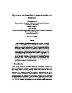
Figure 1: Constraint representation and constraint satisfaction. Given a set of constraints with their selected output variables, the constraint network is viewed as a directed bipartite graph. This graph is referred to as a solution graph. Consider, for example, the four-bar mechanism in Fig. 2(a) where Bar1 is xed. This gure represents a simple design problem (adapted from [Grosjean91]), where the length of each bar is given by d, a, b and c. From Fig. 2(a) the Freudenstein's equation [Grosjean91], which relates the input angle  to output angle as a function of the sizes of the linkages, is expressed as: k1cos + k2cos ? k3 = cos( ? ) (1) where, c1 : k1 = d=c; (2) c2 : k2 = d=a; (3) 2 2 2 2 c3 : k3 = (a ? b + c + d )=2ac: (4) (a)

Bar3 b

Bar2

a c

θ

Bar4 ψ

d Bar1

(b)

k1 100 c1

d

c 120

110 k2

c2

c3

a

b

k3

Figure 2: Four-bar linkage and a solution subgraph. The solution graph, which consists of constraints c1, c2 and c3, is shown in Fig. 2(b). In this graph, numbers attached to each constraint node (i.e., 100, 110 and 120) indicate 5

the current increasing order of constraint satisfaction. Thus, according to Fig. 2(b), the order for satisfying the constraints is: c1, c2 and c3. Note that it makes sense to satisfy constraint c1 before constraint c2, since variable d is an input variable for c2 and an output for c1. The purpose of the INCES algorithm is to incrementally update the constraint dependency and the sequence of satisfaction of the solution graph, when a constraint is inserted or deleted. Section 3.3 explains how INCES achieves this purpose.

3.1.2 Constraint Satisfaction A constraint is said to be satis ed when the value of its output variable is calculated. INCES provides dierent constraint satisfaction techniques, according to a constraint's linearity. Each linear constraint is associated with methods which are used to satisfy the constraint. These methods are procedures that read the values of the input variables and calculate the value of the output variable [Zanden92, Sannella93, Hosobe et al. 94]. For example, given c1 : a = b + c, in Fig. 1, this constraint can be satis ed by any of the following methods : a b + c, b a ? c or c a ? b (see Fig. 3). On the other hand, if the constraint is a non-linear constraint, then it is symbolically processed according to its output variable and solved through the NAG-Fortran library. If a non-linear constraint presents more than one solution, the user is required to choose one of them. (a)

(b)

b

b c1

c

a

c1

a=b+c

c

a

b=a-c

(c) b c1 c

a

c=a-b

Figure 3: Satisfaction methods for c1 : a = b + c

3.2 Local Propagation Techniques Local Propagation [Brunkhart94, Sannella94] is an ecient method for solving systems of constraint equations. After the value  of an unknown variable x is de ned, the method works by propagating its value to all constraints in the constraint network that depend upon x. After substituting the value into the constraints x belongs to, local propagation now examines each of these constraints to see whether only one unknown remains. If so, the constraint is solved and the value of the unknown is calculated. Then the method is recursively applied with the newly acquired value to the remaining network until all constraints are satis ed. However, Local Propagation is only eective for systems of constraints that can be ordered into lower triangular form [Brunkhart94]. Fig. 4 shows two triangular systems. Such systems are best solved using back-substitution, which is the Local Propagation method recursively applied from the bottom constraint to the top one. 6

x ? 3y + 2z + 5w = 4 y + 5z + 3w = 2 3z + 2w = 0 w=3 2 3 2 x + 4y ? 2z + 3w = 2 2y2 + ? w = 0 3z3 =8 2 w =5 Figure 4: Two triangular systems. Therefore, a necessary and sucient condition to solve a set of constraints through Local Propagation is that of having a constraint with only one remaining variable, whenever known values are propagated to the constraint network. If such an unknown variable cannot be identi ed it means that the constraint network has a set of constraints which must be solved simultaneously (a constraint cycle). Fig. 5 shows a system of constraints which can not be triangularized and therefore forms a constraint cycle.

x ? 3y x + 2y +

+ 5w

=4 ? 3t = 0 3z + 2w ? 5t = 2 2z ? 3w + 2t = 3 5z + 4w ? 3t = 5 Figure 5: A Constraint cycle. Thus, when using Local Propagation each variable is set as the output for only one constraint. It should be noted that constraint cycles can not be solved using local propagation techniques. The INCES algorithm starts working by incrementally updating the solution graph through Local Propagation. This process is implemented in two phases :

 a planning phase that selects the output variables for each constraint and identi es the constraint network satisfaction sequence or constraint satisfaction plan. A constraint satisfaction plan is a sequence c1; c2; :::; c of constraints such that c1 is solved before c2, c2 is solved before c3 and so on;  an execution phase that performs the back-substitution necessary to solve the constraints. n

However, if constraint cycles are identi ed during the planning phase, a numerical solution is required. This procedure is explained in Section 3.4.

3.3 Incremental Constraint Insertion As already pointed out, previous approaches [Owen91, Serrano-Gossard92, Kramer92, Brunkhart94] would rebuild the solution graph from scratch, whenever a new a con7

straint is inserted. Therefore, for very large constraint networks, the constraint satisfaction process is time-consuming, making such systems less suitable for interactive design [Zanden92, Fa93]. In order to reduce the time in nding solutions, INCES accommodates the new constraints by incrementally updating the solution graph. This section presents the techniques used by INCES to achieve such incremental graph updating.

3.3.1 Inserting Constraints With Free Variables As mentioned in the previous section, it is crucial when using Local Propagation to have variables which belong to only one constraint in the remaining constraint set. These variables are called free variables. (a)

a 100

c1

c

200

d

c2

b c4

e

h

f

300

c3 g

(b)

a 100

c1

c

200

d

c2

b

250

c4

e

h

300

f

c3 g

Figure 6: Inserted free-variable constraint and its updated solution graph. When a constraint is inserted, INCES rst tries to identify a free variable in this constraint. If such a variable is found it is set as the output of the inserted constraint. For example, in Fig. 6(a) the user inserts constraint c4 into the solution graph, which currently consists of constraints c1, c2 and c3. In this case, the variable h is a free variable for the constraint c4. Therefore, the algorithm sets this variable as the output of constraint c4. If more than one free variable is found, the algorithm chooses any one to be the output. The next step is to insert the constraint in the constraint satisfaction plan. Note that, a constraint can only be satis ed if the values of its input variables are provided. Thus, this new constraint must be satis ed after the constraints which calculate the value of its input variables. Therefore, c4 must be satis ed after c1 and c2 and hence the new constraint satisfaction plan is c1, c2, c4 and c3. The numbers on the constraint nodes have been updated to re ect the new constraint satisfaction plan (Fig. 6(b)). 8

3.3.2 Inserting Constraints Without Free Variables Under certain situations, the inserted constraint may not have a free variable. For example, consider the solution graph shown in Fig. 7 when one tries to x the value of variable h (constraint c6 : h = 10). Note that variable h is not a free variable, since it belongs to constraints c6, c4 and c5. g

e

b

100 110

c1

a

a=b+c

120

d

c2

d=f-g

a=d/e

c

c3

130

j

140

c4

h

c5

Ancestor subgraph

f=h

h=i+j

i

f

c6

Figure 7: An ancestor subgraph. In this case, the INCES algorithm identi es which part of the current solution graph will be aected by the constraint insertion. If the set of constraints in this subgraph can be triangularized together with the inserted constraint, the algorithm locally updates the constraint dependency in this subgraph, through Local Propagation. The aected subgraph is composed only of the nodes that are ancestors of the inserted constraint's variables (ancestor subgraph). A node v is called an ancestor of node w if there is a directed path from v to w. Fig. 7 shows the ancestor subgraph of variable h (dashed ellipse), due to the insertion of constraint c6. This means that the set of constraints which can be triangularized with the inserted constraint c6 are those inside the ancestor subgraph. However, sometimes only part of the ancestor subgraph can be used to satisfy the inserted constraint. This is explained below in detail. (a)

(b)

g d d=f-g

c6

g d

c3

h = 10

h

d=f-g

c6

c3

h = 10

c4

f=h

f

h

(c)

c4

f=h

f

(d) c6

c6

h = 10

h

h = 10

c4

f=h

f

h

Figure 8: Local propagation during solution graph construction. When INCES does not nd a free variable in the inserted constraint, it starts to construct 9

the ancestor subgraph for the inserted constraint. The construction of ancestor subgraph is explained by the arc ow in Fig. 7. Constraint c6 is rst inserted into the ancestor subgraph. To note, a constraint node is always inserted with its associated variable nodes. Therefore, variable h is inserted with c6. In turn, constraint c4 is inserted since it is the ancestor constraint node for h (h is c4's output variable). Then, c3 is inserted by f (Fig. 8(a)). During this construction, the INCES algorithm checks for constraints with free variables, in order to \absorb" the new constraint. For example, as the construction reaches c3, the algorithm detects that g is a free variable, since it only belongs to c3. Thus, the algorithm triggers the Local Propagation process, by making g the output of constraint c3. Subsequently, the constraint dependency is updated as in Fig. 8(b). Constraint c3 is considered solved and is eliminated from the current ancestor subgraph. g

e

b

100 110

c1

a

a=b+c

120

d

c2

d=f-g

a=d/e

c

c3

115

j

140

h

c5 i

c4

f

f=h

h=i+j

c6 114

Figure 9: Updated solution graph after c6 insertion Next, the elimination of constraint c3 causes c4 to have f as a free variable in the ancestor subgraph. Then, Local Propagation continues by setting f as the output for c4 (Fig. 8(c)). The algorithm takes care to insert c4 before c3 in topological order, because f is now one of c3's input variables. Then c4 is also eliminated. Finally, variable h eliminates constraint c6 (Fig. 8(d)). Thus, the solution graph can be updated without the need to visit other ancestor variables such as those belonging to c2 and c1. Fig. 9 shows the updated solution graph. If such free variable cannot be found in the ancestor subgraph, the inserted constraint cannot be eliminated through Local Propagation. This means that the constraint network contains cycles. Section 3.3.4 explains how INCES handle this situation.

3.4 INCES's Approach for Handling Constraint Cycles If an inserted constraint is not eliminated through the Local Propagation process presented in the previous section, the algorithm deduces that the inserted constraint has caused the constraint network to have a cycle. This cycle is composed of the set of constraints which were not eliminated from the ancestor subgraph. When this is the case, the INCES algorithm locally solves this set of simultaneous constraints. To illustrate this, consider the following case study extracted from [Serrano-Gossard92]. The example presents the problem of designing a cantilever beam. The engineering con10

straints are presented below and their respective geometry is shown in Fig. 10. c1 :  ? MY (5) I =0 c2 : M ? FL = 0 (6) 3 (7) c3 : I ? WH 12 = 0 (8) c4 : Y ? H2 = 0 c5 : K ? 3LEI3 = 0 (9) 2 FL (10) c6 :  ? EI = 0  is the bending stress in the beam, I is the cross sectional area moment of inertia, M is the maximum bending moment due to the load F, Y is the distance from the neutral axis to a ber on the surface of the beam, K is the stiness of the beam and E is the Young's modulus of elasticity. L, H and W are the length, height and width of the beam, respectively.  is the slope of the beam. The problem is to identify the values of the dimensions L, H and W, given , M, E, K and . F H

W

L

Figure 10: Geometry for the cantilever beam problem. Serrano [Serrano-Gossard92] presents an approach that solves this problem by automatically deriving a dependency relationship between the unknown variables and the constraints. The constraint network is represented by a directed graph where nodes represent variables and arcs represent constraints. After deriving the dependency between variables and constraints, the graph is traversed in order to identify constraint cycles which are treated as strongly connected components. However, any time a constraint is inserted, the user has again to specify the set of unknown variables and thus the dependency relationship is derived from scratch. Besides, the entire graph is again traversed in order to identify constraint cycles. This section shows how the INCES algorithm has overcome these limitations by allowing the incremental insertion of constraints and also by locally identifying and handling constraint cycles. The algorithm allows the user to insert each constraint and updates the solution graph incrementally as shown in Section 3.3. Fig. 11 shows the current solution graph when one tries to x the value of variable K (constraint c10), after xing the values of , M and E, through constraints c7, c8 and c9. As can be noted, the ancestor subgraph (dashed ellipse) will not have a free variable in this case. Thus, this is the set of constraints that will have to be solved simultaneously. 11

1040

Y

c4

H

1000

σ

1050

c1

c3

W

c10 K

950

c8

M 960 1200

c2

c5

I

L

F

990

980

c6

970

c9 E

φ

c7

Figure 11: Current solution graph before xing the value of K . INCES relies on numerical techniques (Newton-Raphson iteration method) to provide the solution for a cycle of constraints. However, in order to provide a more ecient solving, the algorithm tries to reduce the size of the Jacobian matrix which is decomposed during each iteration of Newton-Raphson [Kahaner et al. 89]. First, the algorithm traverses the ancestor subgraph and eliminates those constraints which x the value of a variable (FixValue constraint, c : v = ;  2 n, it is said to be over-constrained which means that the user has added more constraints to a fully constrained network. Identifying and correctly solving such cases is very important in real-world design [Keirouz et al. 93]. Besides, under- and over-constrained networks re ect a non-valid dimensioning scheme and thus the algorithm would not be able to eciently rely on a numerical solver, since the Jacobian matrix will be singular in both cases [Light-Gossard82]. In order to illustrate an under-constrained cycle, consider Fig. 15 where one again tries to x the value of K . As can be seen, the number of constraints is smaller than the number of variables. In this case, the algorithm asks the user to x one of the variables according to his/her own criteria. After xing the value of the variable, INCES creates a MacroConstraint with the remaining variables inside the cycle and solves it numerically. Before writing the MacroConstraint as a node in the solution graph, INCES presents the calculated values to the user in order to check whether the results are satisfactory. If so, the graph is rewritten with the MacroConstraint. If not, the user is allowed to test other results iteratively. For over-constrained cycles the user is asked to delete redundant constraints. 1040

Y

σ

c4

H

1000 1050

c1

c3

W

c10 K

950

c8

M 1100

1200

c2

c5

I

L

F

1150

c6 E 1140

φ

c7

Figure 15: Under-constrainted cycle 14

Since INCES locally identi es a subset of constraints which is under- or over-constrained, it is able to provide ecient debugging tools to help the user analyse and handle such situations. This approach is more appropriate for interactive design than previous systems which identi es under- and over-constrained networks by considering the entire constraint graph [Light-Gossard82, Serrano-Gossard92].

4 Conclusions and Future Work The ability of a constraint-based variational design system to support interactive design is dependent on its eciency in satisfying constraints. This paper presents an incremental algorithm to speed up the design constraint satisfaction process. A directed bipartite graph is used to represent the constraint network. This graph is incrementally updated when linear or non-linear constraints are inserted. Linear constraints are satis ed through pre-de ned satisfaction methods whereas non-linear constraints are symbolically processed and satis ed by a numerical solver. The attachment of methods to linear constraints allows the constraints to be easily satis ed according to the method procedures. This makes INCES faster than previous approaches which rely entirely on numerical techniques for constraint satisfaction [Lin et al. 81, Serrano-Gossard92]. In addition, by supporting non-linear constraints, INCES is able to solve a wider range of problems than previous incremental linear constraint satisfaction techniques [Zanden92, Hosobe et al. 94]. Most importantly, INCES incrementally identi es and solves constraint cycles. In addition, by locally identifying and handling over- and under-constrained situations, the algorithm increases its feasibility to eectively support Variational Design in relation to previous approaches which identify the same situations by evaluating the whole constraint network. Thus, the algorithm is more suitable to support interactive conceptual design. As future work, techniques will be developed to support direct manipulation with the under-constrained models by exploiting their degrees of freedom. Debugging tools will be developed to provide feedback to the designer for analysing under- and over- constrained situations. Since the potential for user input error is increased with larger constraint networks, it is crucial to help the user to understand the behaviour of constrained models and also to determine why a given solution is produced [Keirouz et al. 93, Heydon-Nelson94, Sannella94]. Furthermore, INCES will be extended to provide inequality constraints in order to support a wider range of design problems.

5 Acknowledgements The authors would like to thank Dr. M. Fa for his support, helpful comments and suggestions. Thanks are due to our colleagues in Constraint-based Modeling Group at Leeds for their many useful discussions. In particular, the help and contribution of A. Munlin, Y. Tsai and S. Carden is much appreciated. Thanks are also due to Dr. Jim Baxter and Brian Henson from the Mechanical Engineering Department in Leeds for their many useful comments on the early draft of this paper. E. Lamounier gratefully acknowledges nancial support from the Brazilian Government through the CAPES foundation.

15

References [Borning et al. 92] Borning, A., Freeman-Benson, B., Wilson, M. 1992 - Constraint Hierarchies, Lisp and Symbolic Computation, Vol. 5, no 3, September, pp 223-270. [Bouma et al. 93] Bouma, W. et al. 1993 - A Geometric Constraint Solver, Technical report CSD-TR-93-054, Department of Computer Science/Purdue University. [Brunkhart94] Brunkhart, Mark, K. 1994 - Interactive Geometric Constraint Systems, Master's thesis, Computer Science Division/University of California, Berkeley. [Buchanan-Pennington93] Buchanan, S.A., de Pennington, A. 1993 - Constraint De nition System: a Computer-algebra based Approach to Solving Geometric-constraint Problems, Computer-Aided Design, Vol. 25, no 12, December, pp 741-750. [Chung-Schussel89] Chung, J., Schussel, M. 1989 - Comparison of Variational and Parametric Design, Proceedings of Autofact'89, pp 5/27-5/44. [Cormen et al. 94] Cormen, T. H., Leiserson, C.E., Rivest, R.L. 1994 Introduction to Algorithms, The MIT Press, Cambridge, Massachusetts, USA. [Dohmen94] Dohmen, M. 1994 - Constraint Techniques in Interactive Feature Modeling. Technical report 94-16, Faculty of Technical Mathematics and Informatics/Delft University, [Fa93] M. Fa., Fernando, T., Dew, P. M. 1993 - Interactive Constraint-based Solid Modelling using Allowable Motion. ACM/SIGGRAPH Symposium on Solid Modeling Foundations and CAD/CAM Applications, May, pp 243-252. [Freeman-Benson et al. 90] Freeman-Benson, B., Maloney, J., Borning, A. 1990 - An Incremental Constraint Solver, Communications of the ACM, Vol. 33, no 1, January, pp 54-63. [Gleicher93] Gleicher, M. 1993 - Practical Issues in Graphical Constraints, First Principles and Practice of Constraint Programming Workshop (PPCP'93), Newport, RI. [Gossard et al. 88] Gossard, D.C., Zuante, R.P., Shakurai, H. 1988 - Representing Dimensions, Tolerances and Features in MCAE Systems, IEEE Computer Graphics and Applications, March, pp 51-59. [Grosjean91] Grosjean, J., 1991 - Kinematics and Dynamics of Mechanisms, McGraw-Hill Book Company Ltd, London, England. [Heydon-Nelson94] Heydon, A., Nelson, G., 1994 - The Juno-2 Constraint-Based Drawing Editor, SRC Research Report 131a, December. [Hosobe et al. 94] Hosobe, H. et al. 1994 - Locally Simultaneous Constraint Satisfaction. Second Principles and Practice of Constraint Programming Workshop (PPCP'94), Washington, USA. [Kahaner et al. 89] Kahaner, D., Moler, C., Nash. S., 1989 - Numerical Methods and Software. Prentice Hall, Englewood Clis, NJ. [Keirouz et al. 93] Keirouz, W.T., Pabon, J., Young, R. 1993 - Exploiting Constraint Dependency Information for Debugging and Explanation, First Principles and Practice of Constraint Programming Workshop (PPCP'93), Newport, RI. 16

[Kramer92] Kramer, G. A., 1992 - A Geometric Constraint Engine, Arti cial Intelligence, Vol. 58, December, pp 327-360. [Light-Gossard82] Light, R., Gossard, D., 1982 - Modi cation of Geometric Models through Variational Geometry, Computer-Aided Design (CAD), Vol. 14 no 4, July, pp 209-214. [Lin et al. 81] Lin, V.C., Gossard, D.C., Light, R.A., 1981 - Variational Geometry in Computer Aided Design, ACM Computer Graphics (SIGGRAPH'81), Vol. 15 no 3, August, pp 171-175. [Lucas et al. 95] Lucas, W. K, Kim Roddis, W.M, Brown, F. M., 1995 - Constraint-Based Reasoning for Structural Concrete Design and Detailing, Constraint-95: Workshop on Constraint-Based Reasoning, FLAIRS-95, April. [Mantyla90] Mantyla, M., 1990 - A Modeling System for Top-Down Design of Assembled Products, IBM Journal of Research Development, Vol. 34 no 5, September, pp 636659. [Owen91] Owen, J.C., 1991 - Algebraic Solution for Geometry from Dimensional Constraints, ACM/SIGGRAPH Symposium on Solid Modeling Foundations and CAD/CAM Applications, June, pp397-407. [Pabon et al. 92] Pabon, J., Young, R., Keirouz, W., 1992 - Integrating Parametric Geometry, Features and Variational Modelling for Conceptual Design, International Journal of System Automation: Research and Applications (SARA), Vol. 2, pp 1732. [Requicha-Rossignac92] Requicha, A. A. G., Rossignac, J. R., 1992 - Solid Modelling and Beyond, IEEE Computer Graphics and Applications, September, pp 31-44. [Rossignac91] Rossignac, J. R., 1991 - Through the Cracks of the Solid Modeling Milestone, Eurographics'91 State of the Art Report on Solid Modeling, pp 23-109. [Sannella93] Sannella, M., 1993 - The SkyBlue Constraint Solver and Its Applications, First Principles and Practice of Constraint Programming Workshop (PPCP'93), Newport, RI. [Sannella94] Sannella, M., 1994 - Analyzing and Debugging Hierarchies of Multi-Way Local Propagation Constraints, Second Principles and Practice of Constraint Programming Workshop (PPCP'94), Washington, USA. [Serrano-Gossard92] Serrano, D., Gossard, D., 1992 - Tools and Techniques for Conceptual Design, In Arti cial Intelligence in Engineering Design Vol. I, E. by C. Tong and D. Sriram, pp 71-116. [Stephanopoulos87] Stephamopoulos, G., 1987 - A Knowledge-Based Framework for Process Design and Control, NSF-AAI Workshop on Arti cial Intelligence in Process Engineering Columbia University, New York, N.Y, March 9-10. [Wilde86] Wilde, D. J., 1986 - A Maximal Activity Principle for Eliminating Overconstrained Optimization Cases, Journal of Mechanisms, Transmissions, and Automation Design / Transactions of the ASME, Vol. 108, September, pp 312-314. 17

[Wolter-Chandrasekaran91] Wolter, J., Chandrasekaran P., 1991 - A Concept for a Constraint-based Representation of Functional and Geometric Design Knowledge, ACM/SIGGRAPH Symposium on Solid Modeling Foundations and CAD/CAM Applications, pp 409-418. [Zanden92] Vander Zanden, B. T., 1992 - A Domain-Independent Algorithm for Incrementally Satisfying Multi-Way Constraints. Technical report CS-92-160, Computer Science Department/University of Tennessee.

18