1
INCREMENTAL MAPPING: THEORETICAL SOLUTION FOR PHOTOGRAMMETRY IN CLOUDY AREAS (English Version of the original in Portuguese: Mapeamento incremental: solução teórica para fotogrametria em áreas nubladas) Please, to reference this paper: SILVA, DANIEL CARNEIRO DA, DALMOLIN, QUINTINO. Mapeamento Incremental: Solução Teórica para Fotogrametria em Áreas Nubladas. Boletim de Ciências Geodésicas. ISSN: 1982-2170. v. 8, p. 55-66, 2002. Available in: http://revistas.ufpr.br/bcg/article/view/1420
2
INCREMENTAL MAPPING: THEORETICAL SOLUTION FOR PHOTOGRAMMETRY IN CLOUDY AREAS Mapeamento incremental: solução teórica para fotogrametria em áreas nubladas Prof. Dr. DANIEL CARNEIRO DA SILVA1 Prof. Dr. QUINTINO DALMOLIN2 1 Universidade Federal de Pernambuco Departamento de Engenharia Cartográfica Ave. Acadêmico Hélio Ramos, S/N 50670-901 Recife, PE e-mail:
[email protected] 2 Universidade Federal do Paraná Curso de Pós Graduação em Ciências Geodésicas Centro Politécnico- Jardim da Américas Curitiba, PR e-mail:
[email protected]
SUMMARY The cloudiness problem in photogrammetry occurs systematically around the globe, mainly in tropical and mountainous regions. In Brazil, there are areas where cloudiness is constant and dense throughout the year, especially in the Northern and Northeastern regions. This fact directly implicates in increases of project costs, due to the great risk of both crew and equipment remaining idled for long periods of time waiting for proper flight conditions. In order to find solutions which use conventional photogrammetry to map these areas, this study shows the results obtained in simulations carried out with the Monte Carlo method, using the algorithm used originally in studies of satellite missions – to which some alterations were introduced – and with cloudiness data obtained from surface stations of meteorological points located at the eastern end of the Northeast of Brazil. The results indicate that the incremental mapping method, similarly in part to the method used with satellite images, significantly reduces the flight time for areas with great cloudiness, or for flights carried out outside ideal seasons. Key Words: Aerial Photogrammetry, Flight Planning, Monte Carlo Method, Cloudiness.
1. INTRODUCTION Cloudiness is the most uncertain factor in a photogrammetric survey mission (Slama, 1980). The planning of photogrammetric flights is based on the knowledge of the frequency of days with completely clear skies, from which the operating time and waiting time on the ground of all crew and equipment will be estimated. This information directly interferes with cost calculations and, depending on the region or time of the year, may make it unviable. Decisions about flights are made daily based on sky observations. If clouds occur on any given locality the only solution is to wait for totally clear weather. Most of the specifications used in Brazil, as well as those recommended by entities such as the International Society of Photogrammetry and Remote Sensing (ISPRS) and the American Society of Photogrammetry (ASP), have very clear clauses stating that photographs with clouds will not be accepted and that portions or sections presenting them shall be flown again. In rare contracts, up to 10% of clouds are allowed. In general, all the specifications of the contract must be obeyed and at most, a few "tentative" flights are carried out. The entire rigor in taking photos is aimed at obtaining the highest quality material possible, although this is practically impossible in certain areas or times of the year. In Brazil, there are areas in the North, Northeast and in the State of Minas Gerais which are especially difficult for photogrammetric surveys due to constant and excessive cloudiness (Regensburg, 1976). The data on favorable cloud conditions for photogrammetric purposes are presented in the form of tables or maps. For Brazil, the following data sources are available: those of Girardi (1975), Chede & Chede (1985), 1º/6º Grupo de Aviação da Aeronáutica (GAV) [1st/6th Airforce Aviation Groups]; and for the Northeast region that of Silva & Dalmolin (2000).
3
There are some methods that can be used in photogrammetry to estimate the on-the-ground waiting time by aircraft and crew, bases on clear sky frequency information, such as that of the Associação Nacional de Empresas de Aerolevantamentos (ANEA) [National Association of Air-survey Companies] or by combinatorial analysis, using only the odds of favorable or unfavorable skies. However, these methods simplify the question by considering that the occurrences are statistically independent and do not allow for more elaborate analyses. In order to solve this question, the present study shows the possibility of adapting the method of simulations initially carried out by NASA in the 1960s (Chang & Willard, 1972; Greaves et al., 1971; Salomonson 1969; Sherr et al., 1968), with the objective of predicting the success of satellite imagery coverage, with regards to cloudiness and time of passage of the satellite over a given area. These studies are based on the simulation method of Monte Carlo (Gilks et al., 1995; Meyer, 1954; Metropolis, 1949). Simulations for photogrammetric surveys should give the flight planner information on the probability of success of executing a service in a particular region and at a certain time of year. The simulations to be carried out require a behavior model of the occurrence of cloud cover. According to Gringorten (1971, 1966), cloudiness can be suitably modeled by Markov chains. Even if the probability distribution (frequency) of the random variable is not normal, the study considers that the variable can be transformed into a new variable Y which obeys the standard normal distribution, expressed by N (0.1). The process to carry out that conformation of variables can be done using the Monte Carlo method, whose working principle is based on the Law of Large Numbers (Ross, 1997). In this present study, the Monte Carlo method was applied to an algorithm originally used for satellite imaging simulations, as shown in section 2. Section 3 describes the changes introduced to adapt the algorithm to the photogrammetric flights, and in section 4 some simulation results are analyzed. Based on these results, it is concluded that a solution for the aerial coverage of low-frequency regions of clear sky is feasible, as it happens in Northeast Brazil, called here incremental mapping. 2. ALGORITHM The simulation method of Sherr et al. (1968) used by Brown (1969), Greaves et al. (1971) and Chang & Willard (1972), was originally developed to estimate satellite imagery success probabilities, in which the area of the image was considered to be equal to the area to be mapped. This algorithm with some adaptations, which will be discussed later, can be applied to photogrammetric flights. The results of the simulations give the odds of success, at a certain level of confidence, and the number of attempts that are required to photograph 100% of the area. The results are presented in the form of graphs. The algorithm was implemented in a program using the Pascal language called MCARLO, which uses as input data the Matrices of Unconditional Probabilities (MUP) and Matrices of Temporal Conditional Probabilities (MTCP), obtained from surface observation (SO) data of cloudiness, from posts of the Instituto Nacional de Meteorologia (INMET) [National Institute of Meteorology], in a period of ten years (from 1989 to 1998). The MUP is a matrix of probabilities (called unconditional only to differentiate it from the conditional), where the lines correspond to the classes of cloud coverage from 1 to 10 (or 10% to 100% overcast); the columns correspond to the months from January to December; and the values correspond to the average frequencies of daily observations – being thus a matrix for the time of 12 and another for 18 UTC (Universal Time Coordinated). The MTCP is a matrix of conditional probabilities among the occurrences of classes on one day and on the next day, in which the lines are the classes that occurred on day n and the columns the classes that occurred on day n+1, being one for each month of the year. Tables 1 and 2 show examples of MUPs of the 12 UTC and 18 UTC, and Tables 3 and 4 show examples of MTCPs, respectively for the stations of the cities of Triunfo and Recife. The Triunfo station is in the north-central part of the state of Pernambuco, and can be considered representative of areas that have favorable seasons for photogrammetric flights, while Recife, which is on the coast, is representative of areas of constant cloudiness. According to Silva (2001), the results of the simulations are representative for a unit of time equivalent to a period of four hours and a unit of area that corresponds to 3,000km2, all according to the characteristics of the data used. In this research study, the number of attempts has the same meaning as the number of consecutive days spent to photograph 100% of an area, or the time, in days, of a successful flight mission. The definition of the size of this standard area is based on the spatial and temporal representativeness of the meteorological data.
4
Table 1. MUP - Matrix of Unconditional Probabilities of Triumph, referring to the 12UTC. 82789 10 20 30 40 50 60 70 80 90 100
12 1 2 19.4 16.0 14.9 16.4 2.8 2.7 8.9 13.3 10.1 10.7 12.1 5.3 11.7 12.9 3.2 7.1 7.7 8.9 9.3 6.7
3 19.8 13.0 3.2 13.8 7.3 8.5 10.9 4.5 8.9 10.1
4 15.7 15.7 1.3 11.7 5.4 9.0 8.1 7.6 13.0 12.6
5 6 7 8 9 10 11 12 22.4 19.1 13.5 29.6 50.5 40.1 35.4 32.0 11.0 6.5 5.3 12.9 12.4 15.1 18.3 18.0 1.1 1.7 3.0 2.2 1.0 5.7 0.8 2.2 7.7 7.8 6.0 4.3 7.6 12.2 11.3 11.5 3.7 4.3 6.4 5.4 6.2 9.0 8.8 9.4 7.7 7.0 6.0 6.5 5.7 6.1 5.4 9.0 5.9 8.7 7.9 9.1 6.7 4.3 8.3 3.6 5.1 4.8 6.4 4.3 2.9 1.4 2.1 2.9 10.3 7.0 7.9 6.5 4.8 3.9 5.8 9.0 25.0 33.0 37.6 19.4 2.4 2.2 3.8 2.5
Table 2. MUP – Matrix of Unconditional Probabilities of Recife, referring to the 18UTC. 82900
18 1 2 1.0 2.5 1.3 2.1 4.8 2.9 7.7 9.6 7.7 11.8 21.6 14.3 17.1 23.6 22.6 13.9 10.0 12.5 6.1 6.8
10 20 30 40 50 60 70 80 90 100
3 2.6 1.6 2.6 10.7 8.4 17.8 22.0 20.7 9.4 4.2
4 1.7 0.7 2.0 5.3 8.0 15.3 21.3 20.3 16.7 8.7
5 1.9 2.3 5.8 4.5 9.0 14.8 22.9 14.8 14.2 9.7
6 0.7 1.0 5.0 6.3 9.3 14.3 15.3 18.0 17.0 13.0
7 1.9 1.9 4.8 3.5 8.1 15.2 16.5 20.0 13.9 14.2
8 2.3 2.6 4.5 5.5 12.7 11.7 20.5 16.9 11.7 11.7
9 2.0 4.7 5.3 7.7 11.3 18.0 20.3 16.3 9.3 5.0
10 2.6 3.2 3.9 6.1 13.9 19.0 22.6 16.1 8.1 4.5
11 0.3 1.7 1.7 6.4 15.5 19.3 22.3 21.3 5.7 5.7
12 0.6 4.2 6.1 8.7 12.6 16.5 22.0 18.4 8.1 2.6
Table 3. MTCP Matrix of Temporal Conditional Probabilities of Triumph, referring to the 12UTC, month of September. 82789 10 20 30 40 50 60 70 80 90 100
9 10 64.7 40.0 100.0 43.8 53.8 50.0 23.1 33.3 10.0 0.0
12 20 10.8 12.0 0.0 12.5 7.7 25.0 15.4 0.0 20.0 20.0
30 1.0 0.0 0.0 6.3 0.0 0.0 0.0 0.0 0.0 0.0
40 6.9 4.0 0.0 0.0 15.4 8.3 7.7 16.7 10.0 20.0
50 3.9 4.0 0.0 6.3 15.4 0.0 15.4 50.0 0.0 0.0
60 4.9 16.0 0.0 0.0 0.0 0.0 7.7 0.0 10.0 0.0
70 3.9 8.0 0.0 25.0 0.0 8.3 7.7 0.0 10.0 0.0
80 2.9 0.0 0.0 0.0 7.7 0.0 7.7 0.0 0.0 20.0
90 1.0 4.0 0.0 0.0 0.0 8.3 15.4 0.0 30.0 40.0
100 0.0 12.0 0.0 6.3 0.0 0.0 0.0 0.0 10.0 0.0
Table 4. MTCP Matrix of Temporal Conditional Probabilities of Recife, referring to the 18UTC, month of October. 82900 10 20 30 40 50 60 70 80 90 100
10 25.0 10.0 0.0 0.0 2.4 0.0 0.0 2.2 4.2 7.7
18 12.5 0.0 0.0 0.0 0.0 8.3 0.0 15.8 2.4 2.4 5.2 5.2 2.9 2.9 4.3 2.2 0.0 0.0 7.7 0.0
12.5 20.0 0.0 0.0 9.5 6.9 5.9 6.5 4.2 0.0
25.0 30.0 16.7 10.5 31.0 12.1 8.8 13.0 0.0 15.4
0.0 30.0 25.0 15.8 19.0 17.2 23.5 19.6 16.7 0.0
25.0 10.0 33.3 15.8 23.8 25.9 23.5 21.7 25.0 7.7
0.0 0.0 16.7 15.8 2.4 15.5 20.6 17.4 37.5 23.1
0.0 0.0 0.0 21.1 4.8 5.2 10.3 8.7 8.3 15.4
0.0 0.0 0.0 5.3 2.4 6.9 1.5 4.3 4.2 23.1
3. MODIFICATIONS IN THE BASIC ALGORITHM The basic algorithm must be adapted to applications for photogrammetric flights, especially in the part related to differences in space and time scales between the image captures, because:
5
Photogrammetric flights get much smaller areas through photographs than the areas imaged by satellite. The passage repeatability of a satellite is of several days while the time of re-flight of a certain flight line may be a few minutes. Satellite images are typically used for small-scale maps and can form mosaics of large areas, with tens of square kilometers, for applications in studies that require little positional accuracy. In the case of aerial photographs the scales are larger, they require stereoscopic covering and are used in the form of blocks. These particularities show that the area surveyed in a photogrammetric flight mission can result in dozens of photographs taken at a more flexible schedule. This is different from the equivalent result obtained from a satellite, which records only one image per passage, at intervals of several days, in fixed times, as is the case for LANDSAT, SPOT or CBERS. In the basic algorithm, three optional routines were implemented to make photogrammetry applications more realistic, namely: 1) random imaging of the area; 2) inclusion of the size of the area to be photographed, according to the surveying project; 3) choice of quantity of classes of coverage considered useful for flights. The first modification suggested by Brown (1970) was the inclusion of the division of the area into one hundred equal parts and the random mapping of that area. This routine generates some random numbers from 1 to 100, which define which parts will be mapped in this attempt. Also are obeyed the clear sky area ratio, the partial increment defined by the cloud class and if each part have had not been mapped in a previous attempt. The process continues until the entire area is mapped. The second modification is the introduction of the size of the area to be surveyed. This is done by informing the percentage of the area to be photographed in relation to the standard area of 3,000 km2. For example, if the area to be photographed is 600 km2, the percentage is 20%. This percentage is marked as a continuous sub-area within the one hundred parts of the total area. This position changes in each mission to simulate the constant alterations in the spatial distribution of the clouds. The completion of this subarea is also random. The introduction of the size of the area is justified by observations and studies that show that as the area decreases, the chances of clear skies increase (Shenk & Salomonson 1971; Kristjansson 1991; Silva 2001). Therefore, the expectation is that the smaller the area, the smaller the number of attempts. The existence of this relation deserves further studies, considering its direct application in photogrammetry and videogrammetry. The third modification is the possibility of including more classes of coverage in addition to class 1. The intention is to flexibly use all percentages of clear areas available in the sky, allowing coverage classes that are more cloudy to be used as well. So, the program has three options: a) class 1, which has 0 to 90% clear sky; b) classes 1, 2 and 3, having 0 to 70% clear sky, which depending on the cloud type, base height and distribution, can increase success chances of the flight, significantly; c) all classes from 1 to 10. The use of all ten classes of sky coverage to take advantage of any cloud-free area implies accepting the idea of incremental mapping or surveying, which was also suggested by Browm (1970). At the end of an incremental surveying the area will be covered by a mosaic, obtained from flights and reflights from which segments of flight lines of various sizes – free of clouds – were used, and which must stereoscopically cover the entire area to be mapped. It should be remembered that cloud formation and duration is a dynamic process (Glass, 1963) that is influenced by the winds (Teagle, 1979). For this reason, it is possible that clouds may occur in a particular flight line and that this same flight line may be re-flown minutes later with a clear sky. The preparation of the mosaic is similar to what is usually done with the satellite images. When one wants to map an area for which one does not have a complete cloud-free image, it is necessary to resort to segments from several other images, even of different times. This procedure, despite having restrictions on photogrammetric service contracts, is not so uncommon. In the day-to-day of airlinesurvey companies, there are many examples of services that were performed by taking advantage of gaps in clear skies, which contain photographs with few clouds. This solution can be used in the cloudier regions. It is certainly not possible to use all the small parts that are free of clouds and shadows, but the larger areas with complete stereoscopic models can form the mosaics. With current techniques – such as photogrammetric flights assisted by the Global Position System-GPS and the Inertial Navigation System-INS (Becker & Barriere, 1993); field support facilities; use of analytical plotters; use of multi-scaling phototriangulation softwares; and the use of correlation techniques of digital photogrammetry images – there are no more absolute restrictions for this
6
kind of survey, which seems to be a viable solution for regions with a lot of cloudiness such as the eastern region of Northeast Brazil (Silva & Dalmolin, 2000).
4. RESULTS OF THE SIMULATIONS Silva (2001) carried out simulations with the MCARLO program using data from 22 stations distributed in the study area in the Northeast of Brazil and analyzed the various modifications introduced in the algorithm. However, this present study will merely present the results for the Triunfo and Recife stations, including only the coverage options of one, three or ten classes. The results of the simulations are given in a number of attempts and in probabilities to photograph 100% of the area. The number of attempts is the number of days spent until the area is fully imaged, since the matrices of conditional probability (the MTCPs) entering the simulation refer to 24-hour intervals. The probabilities that appear in the graphs and tables represent the level of confidence of the result, being that 95% was considered statistically acceptable to define the number of attempts that complete the survey. 4.1 Simulations with variation in the quantity of classes The simulations with a variation of the quantity of classes were carried out with the purpose of evaluating the possibility of reducing the number of attempts, especially in areas with excessive cloudiness. Figures 3 and 4 present the simulations carried out for Triunfo and Recife stations, obtained from the tables generated by the MCARLO program, in which the numbers of attempts and the corresponding probabilities of area to be 100% mapped are shown, considering one, three or ten classes of cloudiness, respective to curves 1c, 3c and 10c. The Triunfo station is located in an area that presents some months (August to December) with a probability of occurrence of class 1 equal to or greater than 30% in the morning. In this case, for September, using class 1, with 95% confidence to photograph 100% of the area, the number of attempts is equal to 6 (Figure 3). When using three classes the number of attempts is 5 and with the ten classes, the trials reduce to 3. The Recife station is in an area of great cloudiness, where the occurrence of class 1 is slightly higher in the afternoon and reaches a maximum of 2.6% in the months of March and October (Table 2). With such low clear sky occurrences the number of attempts grows a lot, as shown by the results of the simulations: when using one class, 164 attempts are needed, when using three classes this is reduced to 56, and it is only by using ten classes of cloudiness that a reasonable number of 5 attempts is obtained.
Figure 3 Example of simulation results for Triunfo station.
Figure 4 Example of simulation results for Recife station
7
From the analysis of similar graphs for the entire Northeast region, Silva (2001) observed the following: 1. The use of ten classes of cloudiness, when compared with the use of class 1, reduces the number of attempts for all regions, being more significant for regions of excessive cloudiness, such as Recife; 2. There was no significant reduction in the number of attempts when classes 1, 2 and 3 were used in all seasons. 3. The exaggerated number of attempts to complete a flight mission in areas of greater cloudiness, such as Recife, shows that it is necessary to have alternative ways of performing flights in these regions, such as incremental surveys using photogrammetry or radar imaging (Mercer, 1995). 4.2 Limitations The estimated time period of four hours will unlikely be fully utilized in a flight attempt, due to factors such as time spent in mobilization, takeoff, climb and travel to the area to be surveyed, flight line positioning procedures, film size limitation and the flight autonomy of the aircraft. Taking all of this into account, the suggestion, to apply the results of the simulations obtained with the algorithm and the alterations introduced in the planning of the photogrammetric flights, should consider the following: a) The simulations are valid to photograph an area S, of variable size and scale, which can be completed in an interval of four hours in a maximum area of up to 3,000 km2. This area S will be the new reference standard area. b) If the entire area can be flown within this interval, the number of attempts obtained in the simulation is directly used. c) If the total area is greater than 3,000 km2, it may be considered that every sub-area S is independent, and thus the number of attempts of the simulation is multiplied by the ratio (total area/standard area). Another suggested solution is to implement the method known as Markovian Scheduling by (Greaves et al., 1971). This scheduling is based on the assumption adopted in the simulation that the occurrences of the clouds are a simple Markov chain and that the matrices of conditional probability for areas N times larger than the reference area are obtained simply by raising the matrices to the N power. 5. CONCLUSIONS The use of a simulation program to stimulate the success of photogrammetric survey missions with the Monte Carlo Method, with the adaptations in the basic algorithm, proved to be viable for the planning of photogrammetric flights, and it even allows for defining levels of reliability of the results. Simulations using the ten coverage classes of cloudiness show a very significant reduction in the number of attempts, suggesting that the use of incremental surveys is a solution to be considered for both the regions of excessive cloudiness – with daily averages above 10% and constant throughout the year – and for surveys carried out in non-ideal seasons. The final survey, consisting of a mosaic of photographs obtained from flights and re-flights totally free of cloudiness, may be used because modern hardware and software techniques allow for multi-scale treatment and processing. 6. REFERENCES 1°/6° Grupo de Aviação. Climatologia Mensal. Recife: Base Aérea, 1°/6° Grupo de aviação, Seção de Informações do Setor de Planejamento Meteorológico. Cartogramas de janeiro a dezembro. 19??. Becker, R. D; Barriere, J. P. Airborne GPS for Photo Navigation and Photogrammetry: An Integrated Approach. Photogrammetric Engineering & Remote Sensing. v. 59, n. 11. p. 1659-1665. Nov. 1993. Brown, S. C. A Cloud-Cover Simulation Procedure. Astronautics & Aeronautics, v. 17, n. 8, p. 86-88. Aug. 1969. ____________. Simulating the Consequence of Cloud Cover on Earth-Viewing Space Mission. Bulletin American Meteorological Society. v. 2, n. 51, p. 126-131. 1970.
8
Chang, D. T; Willard, J. H. Further Developments in Cloud Statistics for Computer Simulations. NASA Contractor Report CR-61389. Alabama: NASA George C. Marshall Space Flight Center, 1972. 109 p. Chede, F. C; Chede, I. C. G. Estudo das Regiões Climatológicas Brasileiras e a sua Utilização Prática na Aerofotogrametria. 2 ed. Rio de Janeiro: Escola de Aperfeiçoamento e Preparação da Aeronáutica Civil. 1985. 45 p. Gilks, W. R; Richardson, S; Spiegelhalter, D. J. Markov Chain Monte Carlo in Practice. Londres: Chapman & Hall. 1995. 486 p. Glass, M. The Growth Characteristics of Small Cumulus Clouds. Journal of the Atmospheric Sciences.v 20. p. 397-406. Sep. 1963. Greaves, J. R; Spiegler, D. B; Willand, J. H. Development of a Global Cloud Model for Simulating EarthViewing Space Missions. NASA Contractor Report CR-61345. Alabama: NASA George C. Marshall Space Flight Center. 1971. 133 p. Girardi, l. C. Áreas e Épocas Favoráveis aos Vôos Aerofotogramétricos. IAE-M-03/73. S. José dos Campos: Centro Técnico Aeroespacial, Instituto de Atividades Espaciais.1973. 22p. Gringorten, I. I. A Stochastic Model of the Frequency and Duration of Weather Events. Journal of Applied Meteorology. V. 5, p. 606-624. Oct. 1966. ________________. Modeling Conditional Probability. Journal of Applied Meteorology. v. 10, p. 646657. Aug. 1971. Kristjansson, J. E. Cloud Parametrization at Different Horizontal Resolutions. Quarterly Journal of Royal Meteorological Society. n. 117, p.1255-1280. 1991. Mercer, J. B. SAR Technologies for Topographic Mapping. In: Photogrammetric Week´95. Karlsruhe: (Ed) Fritsch/Hobbie. Wichmann. p. 117-126. 1995. Metropolis, N. U. The Monte Carlo Method. Journal of the American Statistical Association. v. 44, n. 247, p. 335-341. Sep. 1949. Meyer, A. H. (Ed). Symposium on Monte Carlo Methods. University of Florida: John Wiley & Sons, Inc. 1954. Ratisbona, L. R. The Climate of Brazil. In: Schwerdtfeger, W (Ed). World survey of climatology, volume 12, climates of Central and South America. Amsterdam: Elsevier, v. 12, cap.5, p. 219-294. 1976. Ross, S. M. Introduction to Probability Models. 5th ed. San Diego, EUA: Academic Press, 1993. Salomonson, V. Cloud Statistics in Earth Resouces Technology Satellite (ERTS) Mission Planning. NASA TM X-63674. Mariland, EUA: Goddard Space Flight Center. 1969. 19 p. Shenk, W. E; Salomonson, V. A Simulation Study Exploring the Effects of the Sensor Spatial Resolution on Estimates of Cloud Cover from Satellites. NASA TN-D6247. Mariland, EUA: Goddard Space Flight Center. 1971. 10 p. Sherr, P. E; et al. World Wide Cloud Cover Distribution for use in Computer Simulations. NASA CR 61226. Allied Research Associates, Inc. 1968. Silva, D. C., Dalmolin, Q. Mapa de Céu Claro para uso em Aerofotogrametria. In: Congresso Brasileiro de Cadastro Técnico Multifinalitário- Cobrac 2000. Florianópolis. Anais .... Florianópolis: UFSC. 2000. 1 CD. Silva, D. C. Métodos para Tratamento de Dados de Nebulosidade para Fins Fotogramétricos. Tese de Doutorado em Ciências Geodésicas. Curitiba: Curso de Pós Graduação em Ciências Geodésicas, Universidade Federal do Paraná. 2001. 235 p. Slama, C. C (Ed). Manual of Photogrammetry. 4th ed. Falls Church, VA, EUA: American Society of Photogrammetry. 1980. 1056p. il. Teagle, R. D. Cloud Mapping. In: Preceding of the ASP 45th Annual Meeting. Washington. v. II. p. 524532. 1979.