Incremental multi-class semi-supervised clustering regularized by

Neural Networks 71 (2015) 88–104

Contents lists available at ScienceDirect

Neural Networks journal homepage: www.elsevier.com/locate/neunet

Incremental multi-class semi-supervised clustering regularized by Kalman filtering Siamak Mehrkanoon ∗ , Oscar Mauricio Agudelo, Johan A.K. Suykens KU Leuven, ESAT-STADIUS, Kasteelpark Arenberg 10, B-3001 Leuven (Heverlee), Belgium

article

info

Article history: Received 25 September 2014 Received in revised form 9 July 2015 Accepted 2 August 2015 Available online 14 August 2015 Keywords: Incremental semi-supervised clustering Non-stationary data Video segmentation Low embedding dimension Kernel spectral clustering Kalman filtering

abstract This paper introduces an on-line semi-supervised learning algorithm formulated as a regularized kernel spectral clustering (KSC) approach. We consider the case where new data arrive sequentially but only a small fraction of it is labeled. The available labeled data act as prototypes and help to improve the performance of the algorithm to estimate the labels of the unlabeled data points. We adopt a recently proposed multi-class semi-supervised KSC based algorithm (MSS-KSC) and make it applicable for online data clustering. Given a few user-labeled data points the initial model is learned and then the class membership of the remaining data points in the current and subsequent time instants are estimated and propagated in an on-line fashion. The update of the memberships is carried out mainly using the out-ofsample extension property of the model. Initially the algorithm is tested on computer-generated data sets, then we show that video segmentation can be cast as a semi-supervised learning problem. Furthermore we show how the tracking capabilities of the Kalman filter can be used to provide the labels of objects in motion and thus regularizing the solution obtained by the MSS-KSC algorithm. In the experiments, we demonstrate the performance of the proposed method on synthetic data sets and real-life videos where the clusters evolve in a smooth fashion over time. © 2015 Elsevier Ltd. All rights reserved.

1. Introduction In many real-life applications, ranging from data mining to machine perception, obtaining the labels of input data is often cumbersome and expensive. Therefore in many cases one encounters a large amount of unlabeled data while the labeled data are rare. Semi-supervised learning (SSL) is a framework in machine learning that aims at learning from both labeled and unlabeled data points (Zhu, 2006). SSL algorithms received a lot of attention in the last years due to rapidly increasing amounts of unlabeled data. Several semi-supervised algorithms have been proposed in the literature (Belkin, Niyogi, & Sindhwani, 2006; Chang, Pao, & Lee, 2012; He, 2004; Mehrkanoon & Suykens, 2012; Wang, Chen, & Zhou, 2012; Xiang, Nie, & Zhang, 2010; Yang et al., 2012). However, most of the SSL algorithms, operate in batch mode, hence requiring a large amount of computation time and memory to handle data streams like the ones found in real-life applications such as voice and face recognition, community detection of evolving networks

∗

Corresponding author. Tel.: +32 16328653; fax: +32 16321970. E-mail addresses: [email protected], [email protected] (S. Mehrkanoon), [email protected] (O.M. Agudelo), [email protected] (J.A.K. Suykens). http://dx.doi.org/10.1016/j.neunet.2015.08.001 0893-6080/© 2015 Elsevier Ltd. All rights reserved.

and object tracking in computer vision. Therefore designing SSL algorithms that can operate in an on-line fashion is necessary for dealing with such data streams. In the context of on-line clustering, due to the complex underlying dynamics and non-stationary behavior of real-life data, attempts have been made to design adaptive clustering algorithms. For instance, evolutionary spectral clustering based algorithms (Chakrabarti, Kumar, & Tomkins, 2006; Chi, Song, Zhou, Hino, & Tseng, 2007; Ning, Xu, Chi, Gong, & Huang, 2010), incremental K -means (Chakraborty & Nagwani, 2011), self-organizing time map (Sarlin, 2013) and incremental kernel spectral clustering (Langone, Agudelo, De Moor, & Suykens, 2014). However, in all above-mentioned algorithms the side-information (labels) is not incorporated and therefore they might underperform in certain situations. A semi-supervised incremental clustering algorithm that can exploit the user constraints on data streams is proposed in Halkidi, Spiliopoulou, and Pavlou (2012). The user’s prior information are presented to the algorithm in the form of must-link and cannotlink constraints. The authors in Kamiya, Ishii, Furao, and Hasegawa (2007) introduced an on-line semi-supervised algorithm based on a self-organizing incremental neural network. Here we adopt the recently proposed multi-class semisupervised kernel spectral clustering (MSS-KSC) algorithm

S. Mehrkanoon et al. / Neural Networks 71 (2015) 88–104

(Mehrkanoon, Alzate, Mall, Langone, & Suykens, 2015) and make it applicable for an on-line data clustering/classification. In MSSKSC the core model is kernel spectral clustering (KSC) algorithm introduced in Alzate and Suykens (2010). MSS-KSC is a regularized version of KSC which aims at incorporating the information of the labeled data points in the learning process. It has a systematic model selection criterion and the out-of-sample extension property. Moreover, as it has been shown in Mehrkanoon and Suykens (2014), it can scale to large data. In contrast to the methods described in Adankon, Cheriet, and Biem (2009), Belkin et al. (2006), Chang et al. (2012), Xiang et al. (2010), Yang et al. (2012), in the MSS-KSC approach a purely unsupervised algorithm acts as a core model and the available side information is incorporated via a regularization term. In addition, the method can be applied for both on-line semi-supervised classification and clustering and uses a lowdimensional embedding. In the MSS-KSC approach, one needs to solve a linear system of equations to obtain the model parameters. Therefore with n number of training points, the algorithm has O (n3 ) training complexity with naive implementations. The MSSKSC model can be trained on a subset of the data (training data points) and then applied to the rest of the data in a learning framework. Thanks to the previously learned model, the outof-sample extension property of the MSS-KSC model allows the prediction of the membership of a new point. However, in order to cope with non-stationary data-stream one also needs to continuously adjust the initial MSS-KSC model. To this end, this paper introduces the Incremental MSS-KSC (I-MSS-KSC) algorithm which takes advantage of the available side-information to continuously adapt the initial MSS-KSC model and learn the underlying complex dynamics of the data-stream. The proposed method can be applied in several application domains including video segmentation, complex networks and medical imaging. In particular, in this paper we focus on video segmentation. There have been some reports in the literature on formulating the object tracking task as a binary classification problem. For instance in Teichman and Thrun (2012) a tracking-based semisupervised learning algorithm is developed for the classification of objects that have been segmented. The authors in Badrinarayanan, Budvytis, and Cipolla (2013) introduced a tree structured graphical model for video segmentation. Due to the increasing demands in robotic applications, Kalman filtering has received significant attention. In particular Kalman filter has been applied in wide applications areas such as robot localization, navigation, object tracking and motion control (see Chen, 2012 and references therein). The authors in Suliman, Cruceru, and Moldoveanu (2010) use the Kalman filter for monitoring a contact in a video surveillance sequence. In Zhong and Sclaroff (2003), a Kalman filter based algorithm is presented to segment the foreground objects in video sequences given non-stationary textured background. An adaptive Kalman filter algorithm has been used for video moving object tracking in Weng, Kuo, and Tu (2006). In case of the video segmentation, we show how Kalman filter can be integrated into the I-MSS-KSC algorithm as a regularizer by providing an estimation of the labels throughout the whole video sequences. This paper is organized as follows. In Section 2, the kernel spectral clustering (KSC) algorithm is briefly reviewed. In Section 3, an overview of the multi-class semi-supervised clustering (MSS-KSC) algorithm is given. The incremental multiclass semi-supervised clustering regularized by Kalman filtering approach is described in Section 4. In Section 5, experimental results are given in order to confirm the validity and applicability of the proposed method. The experimental findings and the

89

demonstrative videos are provided in the supplementary material (see Appendix A) of this paper.1 2. Brief overview of KSC The KSC method corresponds to a weighted kernel PCA formulation providing a natural extension to out-of-sample data i.e. the possibility to apply the trained clustering model to outof-sample points. Given training data D = {xi }ni=1 , xi ∈ Rd , the primal problem of kernel spectral clustering is formulated as follows (Alzate & Suykens, 2010): min

w (ℓ) ,b(ℓ) ,e(ℓ)

subject to

Nc −1 1 

2 ℓ=1 (ℓ)

e

N c −1 1 

T

w(ℓ) w (ℓ) −

= Φw

(ℓ)

2n ℓ=1

T

γℓ e(ℓ) Ve(ℓ)

(1)

(ℓ)

+ b 1n , ℓ = 1, . . . , Nc − 1 (ℓ)

(ℓ)

where Nc is the number of desired clusters, e(ℓ) = [e1 , . . . , en ]T are the projected variables and ℓ = 1, . . . , Nc − 1 indicates the number of score variables required to encode the Nc clusters. γℓ ∈ R+ are the regularization constants. Here

Φ = [ϕ(x1 ), . . . , ϕ(xn )]T ∈ Rn×h where ϕ(·) : Rd → Rh is the feature map and h is the dimension of the feature space which can be infinite dimensional. A vector of all ones with size n is denoted by 1n . w (ℓ) is the model parameters vector in the primal. V = diag(v1 , . . . , vn ) with vi ∈ R+ is a user defined weighting matrix. Applying the Karush–Kuhn–Tucker (KKT) optimality conditions one can show that the solution in the dual can be obtained by solving an eigenvalue problem of the following form: VPv Ω α (ℓ) = λα (ℓ) ,

(2) (ℓ)

where λ = n/γℓ , α are the Lagrange multipliers and Pv is the weighted centering matrix: P v = In −

1 1Tn V 1n

1n 1Tn V ,

where In is the n × n identity matrix and Ω is the kernel matrix with ij-th entry Ωij = K (xi , xj ) = ϕ(xi )T ϕ(xj ). In the ideal case of Nc well separated clusters, for a properly chosen kernel parameter, the matrix VPv Ω has Nc − 1 piecewise constant eigenvectors with eigenvalue 1. The eigenvalue problem (2) is related to spectral clustering with random walk Laplacian. In this case, the clustering problem can be interpreted as finding a partition of the graph in such a way that the random walker remains most of the time in the same cluster with few jumps to other clusters, minimizing the probability of transitions between clusters. It is shown that if V = D−1 = diag



1 d1

,...,

1 dn



,

where di = j=1 K (xi , xj ) is the degree of the ith data point, the dual problem is related to the random walk algorithm for spectral clustering. From the KKT optimality conditions one can show that the score variables can be written as follows:

n

e(ℓ) = Φ w (ℓ) + b(ℓ) 1n = ΦΦ T α (ℓ) + b(ℓ) 1n

= Ω α (ℓ) + b(ℓ) 1n ,

ℓ = 1, . . . , Nc − 1. n

The out-of-sample extensions to test points {xi }i=test 1 is done by an Error-Correcting Output Coding (ECOC) decoding scheme. First

1 ftp://ftp.esat.kuleuven.be/stadius/siamak/155-spt.zip.

90

S. Mehrkanoon et al. / Neural Networks 71 (2015) 88–104

the cluster indicators are obtained by binarizing the score variables for test data points as follows: (ℓ)

(ℓ)

qtest = sign(etest ) = sign(Φtest w (ℓ) + b(ℓ) 1ntest )

= sign(Ωtest α (ℓ) + b(ℓ) 1ntest ), where Φtest = [ϕ(x1 ), . . . , ϕ(xntest )]T and Ωtest = Φtest Φ T . The decoding scheme consists of comparing the cluster indicators obtained in the test stage with the codebook (which is obtained in the training stage) and selecting the nearest codeword in terms of Hamming distance. 3. Semi-supervised clustering using MSS-KSC Consider training data points

D = {x1 , . . . , xnUL , xnUL +1 , . . . , xn },





 

Unlabeled (DU )



(3)



+1 −1

Labeled ( DL )

if the ith point belongs to the jth class otherwise.

(4)

The information of the labeled data is incorporated to the kernel spectral clustering (1) by means of a regularization term. The aim of this term is to minimize the squared distance between the projections of the labeled data and their corresponding labels. The formulation of Multi-class semi-supervised KSC (MSS-KSC) described in Mehrkanoon et al. (2015) in primal is given as follows: Q 1

min

w (ℓ) ,b(ℓ) ,e(ℓ)

2 ℓ=1

+ subject to

T

w (ℓ) w(ℓ) −

Q γ1 

2 ℓ=1

T

e(ℓ) Ve(ℓ)

Q γ2  (e(ℓ) − c (ℓ) )T A˜ (e(ℓ) − c (ℓ) )

2 ℓ=1

e(ℓ) = Φ w (ℓ) + b(ℓ) 1n ,

(5)

ℓ = 1, . . . , Q ,

where c ℓ is the ℓ-th column of the matrix C defined as C = [c

(1)

,...,c

(Q )





0nUL ×Q Y

]n×Q =

,

(6)

n×Q

where 0nUL ×Q is a zero matrix of size nUL × Q and Y is defined as previously. The matrix A˜ is defined as follows: A˜ =



0nUL ×nUL 0nL ×nUL

0nUL ×nL In L × n L



,

Q 1

2 ℓ=1

+

+

(7)

Elimination of the primal variables w (ℓ) , e(ℓ) and making use of Mercer’s Theorem (Vapnik, 1998), results in the following linear system in the dual (Mehrkanoon et al., 2015):

    1n 1T R R1n 1T γ2 In − T n c (ℓ) = α (ℓ) − R In − T n Ω α (ℓ) , 1n R1n

1n R1n

(8)

˜ As is shown in Mehrkanoon et al. (2015), where R = γ1 V − γ2 A. given Q labels the approach is not restricted to finding just Q classes and instead is able to discover up to 2Q hidden clusters. In addition, it uses low embedding dimension to reveal the existing number of clusters which is important when one deals with large number of clusters. In fact one maps the data points to a Q dimensional space, which from now on will be referred to as α space, and the solution vectors α (ℓ) (ℓ = 1, . . . , Q ) represent the embedding of the input data in this space. Therefore every point xi (1) (Q ) is associated with the point [αi , . . . , αi ] in the α -space. (space (ℓ) spanned by the solution vector α ). Once the solution to (8) is found, the codebook CB ∈ {−1, 1}p×Q is formed by the unique rows of the binarized solution matrix (i.e. [sign(α (1) ), . . . , sign(α (Q ) )]). Here each code-word is a binary word of length Q and represents a cluster. The maximum number of clusters that can be decoded is 2Q since the maximum value that p can take is 2Q . In the MSS-KSC formulation, the clusters in the projection space (e-space) obtained by e(ℓ) form lines with well-tuned RBF kernel parameters. Whereas the projection of the points in the α -space obtained by α (ℓ) show a localized behavior. (See Mehrkanoon et al., 2015 for more details.) For the sake of clarity we illustrate the projected points in both α and e-spaces, in the case of a synthetic two moons data set in Fig. 1. The MSS-KSC algorithm (Mehrkanoon et al., 2015) is summarized in Algorithm 1. 4. Incremental multi-class semi-supervised clustering

where InL ×nL is the identity matrix of size nL × nL . V is the inverse of the degree matrix defined as previously. Since in Eq. (5) the feature map ϕ is not explicitly known, one uses the kernel trick and solves the problem in the dual. The Lagrangian of the constrained optimization problem (5) becomes

L(w (ℓ) , b(ℓ) , e(ℓ) , α (ℓ) ) =

 ∂L  = 0 → w(ℓ) = Φ T α (ℓ) , ℓ = 1, . . . , Q ,    ∂w(ℓ)     ∂L   = 0 → 1Tn α (ℓ) = 0, ℓ = 1, . . . , Q ,    ∂ b(ℓ) ∂L  = 0 → α (ℓ) = (γ1 V − γ2 A˜ )e(ℓ) + γ2 c (ℓ) ,   ∂ e(ℓ)     ℓ = 1, . . . , Q ,      ∂  L = 0 → e(ℓ) = Φ w(ℓ) + b(ℓ) 1 , ℓ = 1, . . . , Q . n ∂α (ℓ)



where {xi }ni=1 ∈ Rd . The first nUL data points do not have labels whereas the last nL = n − nUL points have been labeled. Assume that there are Q classes (Q ≤ Nc ), then the label indicator matrix Y ∈ RnL ×Q is defined as follows: Yij =

where α (ℓ) is the vector of Lagrange multipliers. Then the Karush–Kuhn–Tucker (KKT) optimality conditions are as follows,

T

w (ℓ) w(ℓ) −

Q γ2 

2 ℓ=1 Q 

ℓ=1

Q γ1 

2 ℓ=1

T

e(ℓ) Ve(ℓ)

(e(ℓ) − c (ℓ) )T A˜ (e(ℓ) − c (ℓ) )

α (ℓ)

T





e(ℓ) − Φ w (ℓ) − b(ℓ) 1n ,

It has been shown in Mehrkanoon et al. (2015) that for the MSS-KSC approach, one has to solve a linear system of size n (number of training data points) in the dual to obtain the cluster membership of the data points. This is fine for batch mode but does not fit practical applications such as on-line semi-supervised clustering, in which the data are entered sequentially. If the distribution of the new arriving data points is not in line with the one of the training points, then the trained model cannot explain well the new distribution. Therefore in those cases an adaptive learning mechanism is required. In what follows we will show how one can use the out-of-sample extension property of the MSS-KSC model for dealing with data streams in an on-line fashion.

S. Mehrkanoon et al. / Neural Networks 71 (2015) 88–104

91

Fig. 1. Two moons data set: The labeled data point of only one class is available and is depicted by the red circle (•). (a): Data points in the original space. (b): The result of MSS-KSC algorithm with RBF kernel. (c): The mapped data points in the α space. (d): The mapped data points in the e space. (For the colored figure, the reader is referred to the web version of this article.)

Algorithm 1: MSS-KSC: (Mehrkanoon et al., 2015)

Semi-supervised

clustering

Input: Training data set D , labels Y , the tuning parameters {γi }2i=1 , the kernel parameter (if any), number of clusters Nc , the test set D test = {xtest }ni=test i 1 and number of available class labels i.e. Q Output: Cluster membership of test data points D test 1

Solve the dual linear system (8) to obtain {α ℓ }ℓ=1 and Q

ℓ Q

2

3

4 5

6

compute the bias term {b }ℓ=1 . Binarize the solution matrix Sα = [sign(α (1) ), . . . , sign(α (Q ) )]n×Q , where α ℓ = [α1ℓ , . . . , αnℓ ]T . p Form the codebook CB = {cq }q=1 , where cq ∈ {−1, 1}Q , using the Nc most frequently occurring encodings from unique rows of solution matrix Sα . (ℓ) Q

Estimate the test data projections {etest }ℓ=1 using (9). Binarize the test projections and form the encoding matrix 1) Q) [sign(e(test ), . . . , sign(e(test )]ntest ×Q for the test points (Here (ℓ) (ℓ) (ℓ) etest = [etest,1 , . . . , etest,ntest ]T ). ∀i, assign xtest to class/cluster q∗ , where i (ℓ) ∗ q = argminq dH (etest,i , cq ) and dH (·, ·) is the Hamming

distance.

4.1. Out-of-sample solution vector In the batch MSS-KSC algorithm (Mehrkanoon et al., 2015), the n cluster membership of new and unseen test points D test = {xi }i=test 1 is done by an Error-Correcting Output Coding (ECOC) decoding scheme. First the cluster indicators are obtained by binarizing the score variables for test data points as follows: (ℓ)

(ℓ)

qtest = sign(etest ) = sign(Φtest w (ℓ) + b(ℓ) 1ntest )

= sign(Ωtest α (ℓ) + b(ℓ) 1ntest ), ℓ = 1, . . . , Q , where Φtest = [ϕ(x1 ), . . . , ϕ(xntest )]T and Ωtest = Φtest Φ T ∈ Rntest ×n , (n is the number of training points). The decoding scheme

consists of comparing the cluster indicators obtained in the test stage with the codebook CB (which is obtained in the training stage) and selecting the nearest codeword in terms of Hamming distance. For an on-line fashion, once the model is built using the training data points, one can use the above procedure to estimate the cluster membership of the new test points. But in order for the model to be able to track the non-stationary changes in the data stream, the initial codebook CB should be adapted on-line so that it has the information of the more recent data points. In addition one has to incrementally update the solution vectors α . Since in the MSS-KSC approach one needs to solve a linear system of equations, it is possible to use for instance the Sherman–Morrison–Woodbury formula (Golub & Van Loan, 2012) to efficiently update the inverse of the coefficient matrix whenever a new data point is arrived without explicitly computing the matrix inverse. In this case, also one should use some decremental algorithm to cope with non-stationary data stream. Here we aim at using the out-of-sample extension capability of the MSS-KSC model. Consider ntest new data points, D test = {xi }ni=test 1 . The score variables are: (ℓ)

etest = Φtest w (ℓ) + b(ℓ) 1ntest = Ωtest α (ℓ) + b(ℓ) 1ntest ,

ℓ = 1, . . . , Q ,

(9)

where Φtest and Ωtest are defined as previously. The third KKT condition in (7),

α (ℓ) = (γ1 V − γ2 A)e(ℓ) + γ2 c (ℓ) ,

ℓ = 1, . . . , Q ,

links the score variables for training, i.e. e, to the solution vector α . The idea now is to extend this link to out-of-sample projections, such that we obtain an out-of-sample solution with localized properties. The out-of-sample solution vector α (ℓ) , ℓ = 1, . . . , Q for the new test data points are then defined as follows: (ℓ) (ℓ) (ℓ) αˆ test , (γ1 Vtest − γ2 Atest )etest + γ2 ctest ,

ℓ = 1, . . . , Q ,

(10)

where ctest consists of label information of some data points. Vtest = 1 1 1 ) is the inverse degree matrix for the test D− test = diag( d , . . . , d 1

ntest

92

S. Mehrkanoon et al. / Neural Networks 71 (2015) 88–104

data points. If there is no label available, one can simply estimate the solution vector by setting ctest and Atest equal zero. In case that the test data set is sampled from the same distribution as the training data points, then the approximated out-of-sample solution vector αˆ test , from Eq. (10), will display localized cluster structures. Thus we have embed the data points xi ∈ Rd into the Q -dimensional Euclidean space called α -space, i.e. (1)

(Q )

xi → αi := (αi , . . . , αi

),

∀i = 1, . . . , ntest .

In the case of well separated clusters, the data points that lie in the same cluster in the original space, are all mapped to one point in α -space. But in practical applications where clusters are not well separated, the data points in the same cluster in the input space will be close to each other in the α -space with respect to the other points in different clusters. Using this localized representation for out-of-sample solutions in α -space it is possible to introduce the representative or conceptual centroid of a cluster in this space. From now on, we use two spaces: the original space X where the data point xi lies and the α -space where the embedded solution vector αi lies. Before starting to introduce the on-line semisupervised clustering algorithm, let us introduce some definitions that will be used in the remaining of the papers. Definition 1. The representative or conceptual centroid of the ith cluster Ai in the X-space, is defined as the mean value of the data points in Ai . We denote the cluster representative in the X-space by repX (Ai ). Definition 2. The representative or conceptual centroid of the ith cluster Ai in the α -space, is defined as the mean value of the embedded solution vector αk∈J , (J = {j |xj ∈ Ai }), across all dimensions of the features. We denote the cluster representative in the α -space by repα (Ai ). Definition 3. A prototype is defined as a point in the X-space or α space that has been labeled. The jth prototype is denoted by prot X,j and prot α,j in X-space and α -space respectively. Definition 4. Assume that the cluster representatives repX (Ai (k)) at time step k are obtained. A new set of data points D (k+1) at time step k + 1 are defined as outliers or in other words they form a new cluster if their kernel evaluations with respect to all training data points are very close to zero. Therefore x∗ ∈ D (k+1) is considered as n outlier if i=tr1 K (x∗ , xi )2 < θ0 where θ0 is a user defined threshold. Furthermore if there is no single data point and prototype assigned to the ith cluster Ai then this cluster is eliminated. In what follows, the on-line semi-supervised algorithm will be described. The proposed on-line multi-class semi-supervised clustering consists of two stages. In the first stage, one trains the MSS-KSC algorithm (Mehrkanoon et al., 2015) using n training data points D (that contains both label and unlabeled data points) to obtain the initial solution vectors αi and the cluster memberships. Assuming that Nc clusters are detected, the initial cluster representative repX (Ai ) and repα (Ai ) are then obtained using Definitions 1 and 2. The aim of the second stage is to predict the membership of the new arriving data points using the updated solution vectors αi . When batch of new data points are arrived the out-of-sample extension properties of the MSS-KSC algorithm is used to approximate the score variables associated with the new points. Next steps composed of the estimation of the projection of the points in the α -space using (10) and calculating the membership of the points. Finally the cluster representatives in both α and X-spaces are updated. (step 13 in Algorithm 2).

Remark 1. If the algorithm is initialized poorly (the first stage), then one cannot expect to have a good clustering performance for the on-line stage (the second stage). The good initialization can be achieved by the aid of user labels and well tuned model parameters. The performance of the initialization can be monitored by checking the value of an internal quality index such as Silhouette, Fisher and Davies–Bouldin indices. Remark 2. The data points that are to be operated can arrive either one-by-one or as a batch of new points. In the proposed I-MSS-KSC algorithm when a batch of new data points arrives at time step k, more than one cluster can be detected without the need of using any extra step (such as applying K -means in the projection space). Given Q cluster representatives at time instant k − 1, the total number of new clusters that can be created at time step k is Q . The binarized projections of the outlier points in the α -space is used as an indicator for the number of new clusters at time instance k. In the case of sequential one-by-one case since at time instance k, only one sample is fed to the algorithm, there will be a possibility of creation of at most one cluster. The proposed on-line semi-supervised clustering algorithm is summarized in Algorithm 2.2 The general stages of the I-MSS-KSC approach are described by the flow-chart in Fig. 2. In Algorithm 2, the data-stream might already have some labeled samples which then can be considered as prototypes. Otherwise, depending on the application, the prototypes can be provided by the user or for instance, for a video segmentation task the prototypes of the objects in motion can be estimated by means of a Kalman filter. 4.2. Computational complexity The computational complexity of the proposed I-MSS-KSC (Algorithm 2) consists of two parts. In the first stage of the algorithm the MSS-KSC is employed to obtain the initial clusters representatives. As in MSS-KSC one needs to solve a linear system of size n × n, therefore the algorithm has O (n3 ) training complexity with naive implementations. In the second stage which corresponds to updating the clusters representatives for the arriving data-stream, mainly computing the kernel matrix, score variables and out-of-sample solutions vectors contribute to the complexity of the algorithm. As in the second stage, the number of training points is ntr = Nc (see step 6 of Algorithm 2), the overall complexity of the second stage of Algorithm 2, neglecting lower order terms, is O (npoints × d × ntr ) with ntr ≪ npoints and d ≪ npoints . Therefore the complexity of the on-line algorithm is linear with respect to the number of datapoints (npoints ) at each time instant. 4.3. Regularizing I-MSS-KSC via Kalman filtering The Kalman filter, also known as Linear Quadratic Estimator (LQE), is an algorithm that provides an efficient computational (recursive) means to estimate the state of a linear dynamical system from noisy measurements, in a way that the variance of the estimation error is minimized. The Kalman filter was introduced in the sixties by Kalman (1960), and it has been successfully applied to the guidance, navigation and control of vehicles, particularly aircraft and spacecraft. In computer vision, the Kalman filter has been extensively used for tracking objects, and it is precisely in this context that we apply this tool in order to generate the labels for

2 A (k) is the ith cluster at time k. i

S. Mehrkanoon et al. / Neural Networks 71 (2015) 88–104

93

Fig. 2. Flow-chart of the incremental multi-class semi-supervised kernel spectral clustering (I-MSS-KSC) algorithm.

further improve this position estimate by using a Kalman filter. We use the following kinetic model to describe the object motion: sx (k) = sx (k − 1) + T vx (k − 1) +

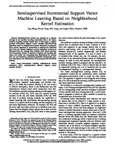
Fig. 3. Kalman filter acts as a regularizer for the MSS-KSC algorithm.

objects in motion. As it can be seen in Eq. (5) the third term of the cost function is influenced by the labels c (ℓ) which are provided by either the user or a Kalman filter. Therefore the Kalman filter is reqularizing the solution of the MSS-KSC through c (ℓ) values associated with the pixels of the objects in motion in a given video sequence. (See the conceptual diagram in Fig. 3.) Consider the following discrete-time linear state-space model of a given dynamical system, x(k + 1) = Ax(k) + Bu(k) + Gw(k)

(11)

y(k) = Cx(k) + v(k) where x(k) ∈ Rnx , u(k) ∈ Rnu and y(k) ∈ Rny are the state, input and output vectors respectively, A ∈ Rnx ×nx , B ∈ Rnx ×nu and C ∈ Rny ×nx are the matrices defining the system dynamics, G ∈ Rnx ×nw is a weighting matrix and w(k) ∈ Rnw and v(k) ∈ Rny are random variables that represent the process (model uncertainties) and measurement (measurement uncertainties) noises respectively. The process noise w(k) is modeled as a Gaussian white noise with zero mean and covariance matrix Q ∈ Rnw ×nw and the measurement noise v(k) is modeled as a Gaussian white noise with zero mean and covariance matrix R ∈ Rny ×ny . Notice that for control and object tracking purposes, it is necessary to know the state vector x(k). However, in general, this vector is not always available. Therefore the use of an estimator such as the Kalman filter becomes necessary in order to provide an estimate of x(k) from the inputs and outputs of the system, on the basis of a mathematical model. The estimate of the state vector x(k) will be denoted by xˆ (k). For the derivation of the Kalman filter equations, readers are referred to Barrero (2005) and Franklin, Powell, and Workman (1990). The Kalman filter is summarized in Algorithm 3,3 where P f (k) is the prior error covariance matrix, xˆ (k) is the estimate of x(k), P (k) is the estimation error covariance matrix and y(k) is a vector comprising the measurements. In this work, we use some image processing techniques to roughly determine the position (measurement) of a moving object for which we would like to provide a label, and afterwards we

3 Here index k denotes the kth frame.

vx (k) = vx (k − 1) + Tax (k − 1) sy (k) = sy (k − 1) + T vy (k − 1) +

vy (k) = vy (k − 1) + Tay (k − 1)

T2 2

ax (k − 1)

T2 2

(12)

ay (k − 1)

where T is the sampling time, sx (k), vx (k) and ax (k) are the position, velocity and acceleration of the object in the x-coordinate, and sy (k), vy (k) and ay (k) are the position, velocity and acceleration of the object in the y-coordinate. If we define the state vector as x(k) = [sx (k), sy (k), vx (k), vy (k)]T , we can write down the kinematic model in a state-space form as follows: x(k + 1) = Ax(k) + Ga(k)

(13)

y(k) = Cx(k) + v(k) where



1 0 A= 0 0

 C =

1 0



0 1 0 0

T 0 1 0

0 T , 0 1

0 1

0 0

0 , 0

T 2 /2  0 G= T 0



0



T /2 , 0 T 2



and a = [ax (k), ay (k)]T . Here it is assumed that ax (k) and ay (k) are normally distributed, with zero mean and standard deviations σax and σay respectively. Observe that there is no Bu(k) term in the previous equations given that there are no control inputs. Finally, the covariance matrices of the process and measurement noise are defined as follows: Q =

 2 σax 0

0

σa2y



,

R=

 2 σmx 0

0

σm2 y



,

where σmx and σmy are the standard deviations of the measured position of the object in the x and y coordinates respectively. These measurements are generated by using some basic image processing techniques (object detection based on color, binarization, computation of centroids, etc.). The interaction between Kalman filter and I-MSS-KSC algorithm is shown in Fig. 4. A video sequence consists of several frames see Fig. 5 and each frame will be treated as batch of new data points for the algorithm.

94

S. Mehrkanoon et al. / Neural Networks 71 (2015) 88–104

Algorithm 2: I-MSS-KSC: On-line Semi-supervised clustering Input: Training data set D , labels Y , the tuning parameters {γi }2i=1 , the kernel parameter (if any), number of clusters Nc , number of prototypes p and number of available class labels i.e. Q Output: Cluster membership of test data points First stage: Initialization of clusters representatives. 1 2

3

Read the training data points (initial set of points, k=1). Train the MSS-KSC model using Algorithm 1 and obtain the cluster membership of the training data points. Calculate the initial cluster representative repX (Ai ) and repα (Ai ) for i = 1, · · · , Nc using Definition 1 and 2. Second stage: Updating the clusters representatives for k=2 to the end of the data-stream do

4

5

6

Read the set of data points (npoints ) at time k, xi (k), i = 1, ..., npoints . Detect the indices of the outlier points according to Def. 4. Provide the prototypes (protα,j (k), j = 1, ..., p) and form the codebook matrix CB for the current k:  time instant   T

CB = repα (Ai (k))



R(Nc +p)×Q .

i=1,...,Nc

  Employ the repX (Ai (k))

 , protα,j (k)



7

∈

j=1,...,p

 as training points and

i=1,...,Nc

calculate the score variables eℓi (k), i = 1, ..., npoints for

Fig. 4. Diagram showing the interaction between Kalman filter and the I-MSS-KSC algorithm for video segmentation purposes. (For the colored figure, the reader is referred to the web version of this article.)

ℓ = 1, ..., Q using (9). 8

9

10

11

12 13

Fig. 5. Some of the frames of the second video sequence. Each slice is treated as a batch of new data points that are fed to the algorithm.

5. Experimental results In this section, some experimental results are presented to illustrate the applicability of the proposed I-MSS-KSC algorithm. In the implementation of Algorithm 2, there are two possibilities:

• I-MSS-KSC (−): the labels (prototypes) are only provided in the first stage, i.e. just for obtaining the initial cluster representatives and the subsequent set of data points do not have any label information. • I-MSS-KSC (+): the user can also provide the labels (prototypes) for some of the subsequent set of data points. In order to illustrate the effect of prototypes (labels), we start with synthetic problems and show the differences between the obtained results when I-MSS-KSC(+) and I-MSS-KSC(−) are applied (see Figs. 6 and 8). Next we show the application of I-MSSKSC reqularized by a Kalman filter to video segmentation. We used RBF kernels for all experiments unless otherwise noted.

Compute the out-of-sample solution vectors αi (k), i = 1, . . . , npoints using (10). Form the encoding matrix for the outlier points by binarizing the obtained αi (k), for all i belonging to the set of outlier indices. . The unique rows of the encoding matrix obtained in step 9, indicates the number of new clusters at time step k. For non-outlier points, assign xi (k) to cluster q∗ , where q∗ = argminj dEuc (αi (k), CB (j, :). Here dEuc (·, ·) is the Euclidean distance and the jth row of the matrix CB is denoted by CB (j, :). Eliminate a cluster if necessary according to Def. 4. Update the cluster representative repX (Ai (k)) and repα (Ai (k)) according to the Definition 1 and 2.

It should be noted that at new time step k, the algorithm can receive either batch of data points or one data point. We first analyze the case that batch of new data points are fed to the algorithm at each time instant. 5.1. Synthetic data sets In Fig. 6, there is a cloud of points which can be clustered in three groups (red, blue and green). The red and green clusters are static over time, whereas the blue cluster is moving toward the other two clusters and then it returns to its initial position. Fig. 6, shows the snapshots of the evolution at specific time instants where one can see the impact of having prototypes in the incremental semi-supervised clustering. At time instants k = 11 and 12, where the blue cluster is close to the other two clusters, there are some points that are not correctly clustered using the I-MSS-KSC(−) algorithm. On the other hand I-MSS-KSC(+) that uses the prototypes (shown by small-squares in Fig. 6) is able

S. Mehrkanoon et al. / Neural Networks 71 (2015) 88–104 Table 1 Averaged ARI index over time for the synthetic data points and time-series.

Algorithm 3: Kalman filter 1

Initialization. Provide the initial guess for state vector xˆ (0) and the estimation error covariance matrix P (0). for

2

k=1 to end do Time update (prediction) Propagate the state vector xˆ (k − 1) one-step ahead,

4

I-MSSKSC(+)

Synthetic data points Synthetic time-series

0.992 0.624

0.999 0.998

P f (k) = AP (k − 1)AT + GQGT

5.2. Synthetic time-series

Measurement update (correction) Compute the Kalman gain,

We show the applicability of the proposed I-MSS-KSC algorithm for on-line time-series clustering. The idea is to cluster signals with similar fundamental frequencies using a sliding window approach. Therefore we have generated two groups of signals with length 600 (each group contains 18 signals) with fundamental frequencies 0.1 rad/s and 0.3 rad/s respectively. Then from time instant k = 200 till k = 400, some of the pure signals of the first group are contaminated with noise which has the same fundamental frequency as the other group. The ground-truth of the time-series are shown in Fig. 8. For I-MSS-KSC, we have labeled one of the pure signals and a contaminated one from the first group. The proposed I-MSS-KSC with and without labels has been applied to cluster the given time-series using a moving window approach. In this experiment the window size was set to 150. To evaluate the outcomes of the model, the average adjusted rand index (ARI) (Halkidi et al., 2001) is used and the results are reported in Table 1. Here the similarity between the time-series is computed using the RBF kernel with the correlation distance (Warren Liao, 2005). The obtained clustering results are compared with the known ground-truth. The snapshots of the obtained results at certain time instants, where the signals from the first group have noise, are depicted in Fig. 9, which shows the advantage of having labels. From Fig. 9, one can observe that when the labels are not provided to the algorithm, it mixes things up, some of the signals from the first group are assigned to the second group and vice versa. However when the prototypes are used by the algorithm, this pattern is not observed.

 −1



Update xˆ f (k) to xˆ (k) by using the measurements y(k), xˆ (k) = xˆ f (k) + L(k) y(k) − C xˆ f (k)



6

I-MSS-KSC(−)

Propagate the covariance matrix P (k − 1) one-step ahead,

L(k) = P f (k)C T CP f (k)C T + R 5

Experiment

six clusters are fed to the algorithm. This number of data points is fixed until time step k = 10 where two clusters are eliminated and therefore the total number of points is 1241 and finally at time step k = 12 another cluster disappears from this step onward the number of data points fed into the algorithm at each step is 1171. The model parameters are γ1 = 1, γ2 = 1 and σ = 1 respectively.

xˆ f (k) = Axˆ (k − 1) + Bu(k − 1) 3

95



Update P f (k) to P (k), P (k) = (I − L(k)C ) P f (k)

to cluster all the data points correctly. Hence incorporating the prototypes helps to improve the performance. In order to evaluate the performance of the two I-MSS-KSC(−) and I-MSS-KSC(+) algorithms quantitatively, the adjusted rand index (ARI) (Halkidi, Batistakis, & Vazirgiannis, 2001) is used and the obtained results are tabulated in Table 1. ARI is an external evaluation criterion which measures the agreement between two partitions and takes values between zero and one. The higher the value of the ARI the better the clustering result is. In this example, at new time step k, the algorithm receives batch of data where the number of data points is the same as that of time step k − 1. Initially at time step k = 1, there are 1191 data points forming three clusters. The total number of labeled data points is 21 and is fixed along all the time steps. The regularization parameters and the kernel bandwidth are γ1 = 1, γ2 = 10−3 and σ = 0.7 respectively. The proposed I-MSS-KSC algorithm is able to detect the creation of more than one new cluster at the given time step k, when batch of new data are fed to the algorithm. In the next example4 , we consider the case that three new clusters are created and eliminated at different time steps. At time step 1, the data set consists of three clusters as in the previous example (see Fig. 7). Three other new clusters (clusters 4, 5 and 6) are created at time step 2. The cluster 4 and 5 are eliminated at time step 10 whereas cluster 6 disappears at time step 12. Definition 4 is used along with the Algorithm 2 and all the above mentioned events are correctly detected. Fig. 7, shows the snapshots of the evolution at specific time instants where clusters are detected and eliminated. A video of this simulation is provided in the supplementary material (see Appendix A) of the paper. The number of data points at time step k = 1 is 1171. In the next step 1371 new data points that form

4 The data set can be found in https://sites.google.com/site/smkmhr/Publications.

5.3. Real-life video segmentation In this section the proposed I-MSS-KSC algorithm is tested on real-life videos5 . We compare the performance of the proposed method with a semi-supervised incremental clustering algorithm (SemiStream) (Halkidi et al., 2012), incremental K -means (IKM) (Chakraborty & Nagwani, 2011) and the Efficient Hierarchical Graph-Based Video Segmentation (EHGB) algorithm proposed in Grundmann, Kwatra, Han, and Essa (2010). The approach described in Halkidi et al. (2012) is an incremental clustering method that exploits the user constraints on data streams in form of must-link and cannot-link constraints. In our experiments, this algorithm is initialized by the MSS-KSC approach (Mehrkanoon et al., 2015). Given the number of constraints we worked with (around 700), it is difficult to evaluate qualitatively the segmentation results when the constraints are displayed. Therefore they are omitted in Figs. 10–13.

5 The data set can be found in https://sites.google.com/site/smkmhr/Publications.

96

S. Mehrkanoon et al. / Neural Networks 71 (2015) 88–104

Fig. 6. Synthetic data sets. On-line semi-supervised clustering using the proposed I-MSS-KSC approach implemented in two modes with and without prototypes (i.e. I-MSSKSC(−) and I-MSS-KSC(+)). First row: The original data points at different time steps. Second row: I-MSS-KSC(−): The results obtained by I-MSS-KSC algorithm without the help of any prototypes after the initialization. Third row: The embedded solution vector α when I-MSS-KSC(−) is applied. Fourth row: I-MSS-KSC(+): The results obtained by the proposed I-MSS-KSC algorithm with the help of prototypes. Fifth row: The embedded solution vector α when I-MSS-KSC(+) is applied. (For the colored figure, the reader is referred to the web version of this article.)

K -means is one of the most popular data clustering methods due to its simplicity and computational efficiency. It works by selecting some random initial centers and then iteratively adjusting the centers such that the total within cluster variance is minimized. In its incremental variant (Incremental K -means), at each time-step it uses the previous centroids to find the new cluster centers, thus avoiding to rerun the K -means algorithm from scratch (Chakraborty & Nagwani, 2011).

The EHGB algorithm is an efficient and scalable technique for spatio-temporal segmentation of long video sequences using a hierarchical graph-based algorithm. The algorithm begins with oversegmenting a volumetric video graph into space–time regions grouped by appearance. Then a ‘‘region graph’’ over the obtained segmentation is constructed and this process is repeated over multiple levels to create a tree of spatio-temporal segmentations (Grundmann et al., 2010). This algorithm comes with some

S. Mehrkanoon et al. / Neural Networks 71 (2015) 88–104

97

Fig. 7. Synthetic data sets. On-line detection of the creation of more than one cluster at time step k using the proposed I-MSS-KSC(+) approach. At time step k = 2, three new clusters appear and evolve. Two of them disappear at time step k = 10 and the third one dies out at k = 12. The labels are just provided for the consistent clusters i.e. the ones that are always present at all the time steps and can possibly evolve over time. The video of this simulation can be found in the supplementary material (see Appendix A) of the paper.

parameters. In all the experiments, we have selected a minimum and maximum number of regions which are stated in the corresponding caption of each of the tested video sequence. Although the EHGB algorithm does not employ labels, it is one of the state-of-the-art algorithms for video segmentation that uses past and future information (in offline mode) in order to segment the current frame. Also this algorithm uses advanced features,

such as color and flow histograms. It should be noted that our algorithm uses the previous segmentation results to perform the segmentation of the current frame. And the algorithm uses only the color feature as discriminator (local color histograms). Four real examples are used to test the validity of the proposed method. The first example shows two bouncing balls and the second example presents a human’s hand throwing a ball upwards.

98

S. Mehrkanoon et al. / Neural Networks 71 (2015) 88–104

Fig. 8. Ground-truth of the time-series. (a) Signals that are in cluster 1, (a) signals that are in cluster 2.

Fig. 9. Synthetic time-series. On-line semi-supervised clustering using the proposed I-MSS-KSC approach implemented in two modes with and without prototypes (I-MSS-KSC(−) and I-MSS-KSC(+)). First row: I-MSS-KSC(−): The signals assigned to cluster 1 using the I-MSS-KSC algorithm without the help of any prototypes after the initialization. Second row: I-MSS-KSC(+): The signals assigned to cluster 1 using I-MSS-KSC algorithm with the help of the prototypes. Third row: I-MSS-KSC(−): The signals assigned to cluster 2 using the I-MSS-KSC algorithm without the help of any prototypes after the initialization. Fourth row: I-MSS-KSC(+): The signals assigned to cluster 2 using I-MSS-KSC algorithm with the help of the prototypes.

S. Mehrkanoon et al. / Neural Networks 71 (2015) 88–104

99

Table 2 Videos statistics. Video

width × height

# batch data points

# of frames

Frame rate (frames/s)

Bouncing ball Siamak’s hand Dominoes Birds

320 × 180 320 × 180 435 × 343 1280 × 720

57 600 57 600 149 205 921 600

139 395 121 162

29 29 29 29

Table 3 The number of quantization levels, unlabeled/labeled training and validation points used to obtain the initial cluster representatives. Video

Bouncing ball Siamak’s hand Dominoes Birds

Quantization level

10 8 15 13

Q

D val

D

3 3 3 4

Du

DL

Duval

DLval

1000 800 600 1000

4 3 3 4

1500 1500 1500 1500

3 3 3 3

The third video is a video sequence taken from Berkeley video segmentation data set6 and is called dominoes video and the fourth video is a high definition video showing birds. Descriptions of the used videos can be found in Table 2. In order to extract features from a given frame, a local color histogram with a 5 × 5 pixels window around each pixel using minimum variance color quantization is computed. The level of quantization in general depends on the video under study. The number of levels used for each of the videos is reported in Table 3. The χ 2 kernel K (h(i) , h(j) ) = exp(−

χij2 σχ2

) with parameter σχ ∈ R+ is

used to compute the similarity between two color histograms h(i) and h(j) . Here χij2 =

1 2

nq

q =1

(i)

(j)

(hq −hq )2 (j) (i) hq +hq

where nq is the number of

quantization levels. The performance of the proposed I-MSS-KSC model depends on the choice of the tuning parameters. We set the regularization parameters γ1 = γ2 = 1 to give equal weights to unlabeled and labeled data points. The initial σχ (kernel parameter) is tuned using a grid search in the range [10−3 , 101 ]. The training and validation data points, i.e. D and D val , consist of the histograms of the chosen pixel (unlabeled data points) together with some labeled data points. These data points are used for training and validation respectively to obtain the initial cluster representatives for the first frame. Then the solution vectors and cluster representatives are updated in an on-line fashion using Algorithm 2 for the subsequent frames. The number of unlabeled/labeled training and validation data points used to obtain the initial cluster representatives are tabulated in Table 3. We obtain the initial model using the MSS-KSC algorithm trained on the first frame and then I-MSS-KSC is applied

6 ftp://ftp.cs.berkeley.edu/pub/projects/vision/BVDS_train.tar.gz.

to segment the upcoming frames in an on-line fashion. For IKM, we let the algorithm to initialize itself and the maximum number of iterations allowed is set to 100. Both qualitative and quantitative evaluations of the proposed approaches are provided. For quantitative evaluation of the video segmentation there is not a unique criterion to evaluate the performance of the algorithm under study. Several evaluation criteria are proposed in the literature (Borsotti, Campadelli, & Schettini, 1998; Tan, Mat Isa, & Lim, 2013). Here two criteria are used to evaluate the segmentation results. In the first criterion the segmentation obtained by I-MSS-KSC, EHGB, IKM and SemiStream are compared in Table 4 with the results of the minimum variance quantization method (the number of levels is defined by the user) (Heckbert, 1982) using the Variation of information (VOI) index. This index measures the distance between two segmentations in terms of their average conditional entropy. Low values indicate good match between segmentations (Arbelaez, Maire, Fowlkes, & Malik, 2011). In the second criterion, the segmentations obtained by the above-mentioned approaches are compared in Table 4 with the original frames using the cluster quality index (CQI) which is empirically defined in the following lines. Suppose for a given image I, the segmented image has Nc clusters (regions). We define the quality index per cluster as follows:

 QIj = 1 −

i∈{R,G,B}

mean(|Pji − mij |) 3

,

j = 1, . . . , Nc ,

where Pji denotes the ith channel of the RGB color for pixels of the original image I that belong to cluster j. mij is the mean value of Pji . Next, the cluster quality index (CQI) for a given image I is heuristically defined as a weighted sum of the quality index per cluster i.e. CQI (I ) =

Nc 

θj QIj ,

(14)

j =1 c where j=1 θj = 1. In our setting the highest weight is assigned to the cluster with minimum QI index. The CQI takes values in the range [0, 1]. The higher the value of the CQI(I) the better the segmentation is. The obtained results of the proposed I-MSS-KSC algorithm (with two modes of implementation: I-MSS-KSC(−) and I-MSS-KSC(+)), Incremental K -means, EHGB and SemiStream for some of the

N

Table 4 Comparison of IKM, SemiStream, EHGB, I-MSS-KSC (−) and I-MSS-KSC (+) in terms of averaged cluster quality and variation of information indices over the number of frames. Video

Evaluation criterion

Method IKM

SemiStream

EHGB

I-MSS-KSC (−)

I-MSS-KSC (+)

Bouncing ball

CQI VOI CQI VOI CQI VOI CQI VOI

0.906 1.17 0.872 1.08 0.843 1.552 0.848 0.564

0.921 0.715 0.918 0.382 0.865 1.581 0.868 0.341

0.875 0.839 0.890 1.118 0.880 1.598 0.874 0.539

0.895 0.912 0.919 0.494 0.855 1.584 0.868 0.376

0.924 0.627 0.925 0.344 0.866 1.352 0.868 0.376

Siamak’s hand Dominoes Birds

Note: The higher the value of CQI index the better the segmentation is. The lower the value of VOI, the better the segmentation is.

100

S. Mehrkanoon et al. / Neural Networks 71 (2015) 88–104

Fig. 10. Bouncing balls video. On-line video segmentation results using the proposed I-MSS-KSC, IKM (Chakraborty & Nagwani, 2011) and EHGB (Grundmann et al., 2010). First row: The original frames. Second row: The segmentation results obtained by on-line IKM. Third row: The segmentation results obtained by SemiStream approach (Halkidi et al., 2012) initialized with MSS-KSC (Mehrkanoon et al., 2015), Notice that the must-link and cannot-link constraints are not shown. Fourth row: The segmentation results obtained by EHGB approach (Grundmann et al., 2010) with Min/Max Number of regions = 10/200. Fifth row: The segmentation results obtained by the proposed I-MSS-KSC algorithm without the help of any labeled pixels after the first frame i.e. I-MSS-KSC(−) mode. Sixth row: The results of the proposed I-MSS-KSC algorithm when labeled pixels for two clusters are provided during on-line segmentation, i.e. I-MSS-KSC(+) mode.

frames of the bouncing-ball and Siamak’s hand videos are depicted in Figs. 10 and 11 respectively (the videos of these simulations are presented in the supplementary material (see Appendix A) of the paper). Figs. 10 and 11, show that it is possible to improve the performance of the video segmentation by incorporating prototypes. Note that for the first video sequence, one of the ball and the table are the objects of interest. Since the table is static, the labels are provided by the user and they are fixed through out the video sequence. Whereas the ball’s prototype is provided by a Kalman filter. Here one may notice that I-MSS-KSC(+) makes it possible to improve the performance by carrying the object labeled through out the video sequence. The labeled pixels of the objects are shown by red and white asterisks (∗). The obtained results of the proposed method (I-MSS-KSC(+)), IKM, EHGB and SemiStream

for the third video are shown in Fig. 12 (the video of this simulation is provided in the supplementary material (see Appendix A) of the paper). Fig. 12 indicates that the on-line segmentation results can be improved when the labels are incorporated into the algorithm. In Fig. 12, the labeled pixels of the objects are shown by yellow and white asterisks (∗). The segmentation of the Birds video using the above-mentioned algorithms is shown in Fig. 13. In this video at each time instant 921 600 data points are analyzed. 6. Particular case: one-by-one In case that the data points arrive one by one, the proposed algorithm 2 is still applicable but few modifications are needed. Assuming that a new data point xnew is fed to the algorithm, then

S. Mehrkanoon et al. / Neural Networks 71 (2015) 88–104

101

Fig. 11. Siamak’s hand video. On-line video segmentation results using the proposed I-MSS-KSC, IKM (Chakraborty & Nagwani, 2011) and EHGB (Grundmann et al., 2010). First row: The original frames. Second row: The segmentation results obtained by on-line IKM. Third row: The segmentation results obtained by SemiStream approach (Halkidi et al., 2012) initialized with MSS-KSC (Mehrkanoon et al., 2015), Notice that the must-link and cannot-link constraints are not shown. Fourth row: The segmentation results obtained by EHGB approach (Grundmann et al., 2010) with Min/Max Number of regions = 10/200. Fifth row: The segmentation results obtained by the proposed I-MSS-KSC algorithm without the help of any labeled pixels after the first frame, i.e. I-MSS-KSC(−) mode. Sixth row: The results of the proposed MSS-KSC algorithm when labeled pixels for two clusters are provided during on-line segmentation, i.e. I-MSS-KSC(+) mode.

the following formula is used to update the cluster representatives in both X and α -spaces (line 11 of Algorithm 2):

the latter are not linearly separable from each other (Asuncion & Newman, 2007).

repX (Ai (k)) = µ · repX (Ai (k − 1)) + (1 − µ)xnew

Initially the model is trained only using the data points (labeled and unlabeled) from the first two classes. When an unlabeled new data point arrives, the algorithm decides whether the new point belongs to one of the existing classes or a new class should be created. For the experiment conducted on the Wine and Iris data sets, all the arriving new points were unlabeled (I-MSS-KSC(−)).

repα (Ai (k)) = µ · repα (Ai (k − 1)) + (1 − µ)αnew , where µ ∈ [0, 1]. In addition, line 10 of Algorithm 2 which corresponds to cluster elimination is deactivated. We applied the algorithm to two real data sets Iris and Wine from UCI repository. Wine data set contains three types of wine described by three classes. These data are the results of a chemical analysis of wines produced in the same region in Italy but derived from three different cultivators. The Iris data set is composed of three types of iris plant. One class is linearly separable from the other two;

The number of training/test data points and the obtained results over 5 simulation runs are tabulated in Table 5. These data sets are not linearly separable and there is an overlap between two of the classes (class 2 and 3). The creation of the new class is based on the user defined threshold ϵ (see Definition 4). However as we are

102

S. Mehrkanoon et al. / Neural Networks 71 (2015) 88–104

Fig. 12. Dominoes video. On-line video segmentation results using the proposed I-MSS-KSC, IKM (Chakraborty & Nagwani, 2011) and EHGB (Grundmann et al., 2010). First row: The original frames. Second row: The segmentation results obtained by on-line K -means. Third row: The segmentation results obtained by SemiStream approach (Halkidi et al., 2012) initialized with MSS-KSC (Mehrkanoon et al., 2015), Notice that the must-link and cannot-link constraints are not shown. Fourth row: The segmentation results obtained by EHGB approach (Grundmann et al., 2010) with Min/Max Number of regions = 10/100. Fifth row: The segmentation results obtained by the proposed I-MSS-KSC algorithm without the help of any labeled pixels after the first frame i.e. I-MSS-KSC(−) mode. Sixth row: The results of the proposed I-MSS-KSC algorithm when labeled pixels for two clusters (objects) are provided during on-line segmentation. Note that one object is static and therefore its labels will be static and can be provided by the user.

Table 5 The number of unlabeled/labeled training points used to obtain the initial cluster representatives. The averaged accuracy on the test is reported. Dataset

# classes

Dimension

D Du

DL

Iris Wine

3 3

4 13

17 22

33 43

D test

Accuracy

100 113

0.81 ± 0.04 0.90 ± 0.08

in the semi-supervised setting, the possibility of incorporating the user labels of the third class into the algorithm is also an option.

7. Conclusions In this paper, a new incremental multi-class semi-supervised algorithm is proposed. It uses the multi-class semi-supervised kernel spectral clustering (MSS-KSC) as core model. The update of the solution vectors and the memberships are obtained using the out-of-sample solution property of the MSS-KSC approach. The user labels or labels provided by a Kalman filter are incorporated into the algorithm in an on-line fashion to improve the performance of the I-MSS-KSC. The validity and applicability of the proposed method is shown on synthetic data sets

S. Mehrkanoon et al. / Neural Networks 71 (2015) 88–104

103

Fig. 13. Birds video. On-line video segmentation results using the proposed I-MSS-KSC, IKM (Chakraborty & Nagwani, 2011) and EHGB (Grundmann et al., 2010). First row: The original frames. Second row: The segmentation results obtained by on-line K -means. Third row: The segmentation results obtained by SemiStream approach (Halkidi et al., 2012) initialized with MSS-KSC (Mehrkanoon et al., 2015), Notice that the must-link and cannot-link constraints are not shown. Fourth row: The segmentation results obtained by EHGB approach (Grundmann et al., 2010) with Min/Max Number of regions = 10/100. Fifth row: The segmentation results obtained by the proposed I-MSS-KSC algorithm without the help of any labeled pixels after the first frame i.e. I-MSS-KSC(−) mode. Sixth row: The results of the proposed I-MSS-KSC algorithm when labeled pixels for two clusters are provided during on-line segmentation.

and some real-life videos sequences. For the video segmentation test cases, the results obtained by the proposed I-MSS-KSC algorithm is compared with those of the incremental K -means (IKM) (Chakraborty & Nagwani, 2011), the Efficient Hierarchical Graph-Based Video Segmentation algorithm (EHGB) (Grundmann et al., 2010) and the semi-supervised incremental clustering algorithm (SemiStream) (Halkidi et al., 2012). In general our results obtained by the proposed I-MSS-KSC approach outperforms the incremental K -means (IKM) (Chakraborty & Nagwani, 2011) and comparable with the ones of the EHGB approach. In addition as opposed to SemiStream that uses many must-link and cannot-link constrains, we work with few user defined labeled data points (prototypes) which act as attractors for other unlabeled data points.

Acknowledgments

• EU: The research leading to these results has received funding from the European Research Council under the European Union’s Seventh Framework Programme (FP7/2007–2013) / ERC AdG A-DATADRIVE-B (290923). This paper reflects only the authors’ views, the Union is not liable for any use that may be made of the contained information. • Research Council KUL: GOA/10/09 MaNet, CoE PFV/10/002 (OPTEC), BIL12/11T; PhD/Postdoc grants • Flemish Government: ◦ FWO: projects: G.0377.12 (Structured systems), G.088114N (Tensor based data similarity); PhD/Postdoc grants ◦IWT: projects: SBO POM (100031); PhD/Postdoc grants ◦ iMinds Medical Information Technologies SBO 2014 • Belgian Federal Science Policy Office: IUAP P7/19 (DYSCO, Dynamical systems, control and optimization, 2012–2017). Johan Suykens is a professor at the KU Leuven, Belgium.

104

S. Mehrkanoon et al. / Neural Networks 71 (2015) 88–104

Appendix A. Supplementary material The experimental findings and the demonstrative videos associated with this paper can be found in the on-line version at ftp://ftp.esat.kuleuven.be/stadius/siamak/155-spt.zip. Supplementary material related to this article can be found online at http://dx.doi.org/10.1016/j.neunet.2015.08.001. References Adankon, M. M., Cheriet, M., & Biem, A. (2009). Semi-supervised least squares support vector machine. IEEE Transactions on Neural Networks, 20(12), 1858–1870. Alzate, C., & Suykens, J. A. K. (2010). Multiway spectral clustering with out-ofsample extensions through weighted kernel PCA. IEEE Transactions on Pattern Analysis and Machine Intelligence, 32(2), 335–347. Arbelaez, P., Maire, M., Fowlkes, C., & Malik, J. (2011). Contour detection and hierarchical image segmentation. IEEE Transactions on Pattern Analysis and Machine Intelligence, 33(5), 898–916. Asuncion, A., & Newman, D.J. (2007). UCI machine learning repository. Badrinarayanan, V., Budvytis, I., & Cipolla, R. (2013). Semi-supervised video segmentation using tree structured graphical models. IEEE Transactions on Pattern Analysis and Machine Intelligence, 35(11), 2751–2764. Barrero, O. (2005). Data assimilation in magnetohydrodynamics systems using Kalman filtering. (Ph.D. dissertation), Leuven, Belgium: Katholieke Universiteit Leuven (KU Leuven). Belkin, M., Niyogi, P., & Sindhwani, V. (2006). Manifold regularization: A geometric framework for learning from labeled and unlabeled examples. The Journal of Machine Learning Research, 7, 2399–2434. Borsotti, M., Campadelli, P., & Schettini, R. (1998). Quantitative evaluation of color image segmentation results. Pattern Recognition Letters, 19(8), 741–747. Chakrabarti, D., Kumar, R., & Tomkins, A. (2006). Evolutionary clustering. In Proceedings of the 12th ACM SIGKDD international conference on knowledge discovery and data mining (pp. 554–560). ACM. Chakraborty, S., & Nagwani, N. (2011). Analysis and study of incremental k-means clustering algorithm. In High performance architecture and grid computing (pp. 338–341). Springer. Chang, C. C., Pao, H. K., & Lee, Y. J. (2012). An RSVM based two-teachers–one-student semi-supervised learning algorithm. Neural Networks, 25, 57–69. Chen, S. (2012). Kalman filter for robot vision: a survey. IEEE Transactions on Industrial Electronics, 59(11), 4409–4420. Chi, Y., Song, X., Zhou, D., Hino, K., & Tseng, B. L. (2007). Evolutionary spectral clustering by incorporating temporal smoothness. In Proceedings of the 13th ACM SIGKDD international conference on Knowledge discovery and data mining (pp. 153–162). ACM. Franklin, G., Powell, J., & Workman, M. (1990). Digital control of dynamic systems (2nd ed.). Addison-Wesley. Golub, G. H., & Van Loan, C. F. (2012). Matrix computations. Johns Hopkins University Press. Grundmann, M., Kwatra, V., Han, M., & Essa, I. (2010). Efficient hierarchical graphbased video segmentation. In IEEE conference on computer vision and pattern recognition (pp. 2141–2148). IEEE. Halkidi, M., Batistakis, Y., & Vazirgiannis, M. (2001). On clustering validation techniques. Journal of Intelligent Information Systems, 17(2–3), 107–145.

Halkidi, M., Spiliopoulou, M., & Pavlou, A. (2012). A semi-supervised incremental clustering algorithm for streaming data. In Advances in knowledge discovery and data mining (pp. 578–590). Springer. He, X. (2004). Incremental semi-supervised subspace learning for image retrieval. In Proceedings of the 12th annual ACM international conference on Multimedia (pp. 2–8). ACM. Heckbert, P. (1982). Color image quantization for frame buffer display. Vol. 16. ACM, no. 3. Kalman, R. E. (1960). A new approach to linear filtering and prediction problems. Transactions of the ASME. Series D, Journal of Basic Engineering, 82, 34–45. Kamiya, Y., Ishii, T., Furao, S., & Hasegawa, O. (2007). An online semisupervised clustering algorithm based on a self-organizing incremental neural network. In International joint conference on neural networks, (IJCNN 2007). (pp. 1061–1066). IEEE. Langone, R., Agudelo, O. M., De Moor, B., & Suykens, J. A. K. (2014). Incremental kernel spectral clustering for online learning of non-stationary data. Neurocomputing, 139, 246–260. Mehrkanoon, S., Alzate, C., Mall, R., Langone, R., & Suykens, J. A. K. (2015). Multiclass semisupervised learning based upon kernel spectral clustering. IEEE Transactions on Neural Networks and Learning Systems, 26(4), 720–733. Mehrkanoon, S., & Suykens, J. A. K. (2012). Non-parallel semi-supervised classification based on kernel spectral clustering. In The 2013 international joint conference on neural networks (IJCNN) (pp. 2311–2318). IEEE. Mehrkanoon, S., & Suykens, J. A. K. (2014). Large scale semi-supervised learning using KSC based model. In Proceedings of the 2014 IEEE world congress on computational intelligence (IEEE WCCI/IJCNN 2014),July 6-11, 2014, Beijing, China (p. 8). IJCNN. Ning, H., Xu, W., Chi, Y., Gong, Y., & Huang, T. S. (2010). Incremental spectral clustering by efficiently updating the eigen-system. Pattern Recognition, 43(1), 113–127. Sarlin, P. (2013). Self-organizing time map: an abstraction of temporal multivariate patterns. Neurocomputing, 99, 496–508. Suliman, C., Cruceru, C., & Moldoveanu, F. (2010). Kalman filter based tracking in an video surveillance system. Advances in Electrical and Computer Engineering, 10(2), 30–34. Tan, K. S., Mat Isa, N. A., & Lim, W. H. (2013). Color image segmentation using adaptive unsupervised clustering approach. Applied Soft Computing, 13(4), 2017–2036. Teichman, A., & Thrun, S. (2012). Tracking-based semi-supervised learning. The International Journal of Robotics Research, 31(7), 804–818. Vapnik, V. (1998). Statistical learning theory. Wiley. Wang, Y., Chen, S., & Zhou, Z.-H. (2012). New semi-supervised classification method based on modified cluster assumption. IEEE Transactions on Neural Networks and Learning Systems, 23(5), 689–702. Warren Liao, T. (2005). Clustering of time series data—a survey. Pattern Recognition, 38(11), 1857–1874. Weng, S.-K., Kuo, C.-M., & Tu, S.-K. (2006). Video object tracking using adaptive Kalman filter. Journal of Visual Communication and Image Representation, 17(6), 1190–1208. Xiang, S., Nie, F., & Zhang, C. (2010). Semi-supervised classification via local spline regression. IEEE Transactions on Pattern Analysis and Machine Intelligence, 32(11), 2039–2053. Yang, Y., Nie, F., Xu, D., Luo, J., Zhuang, Y., & Pan, Y. (2012). A multimedia retrieval framework based on semi-supervised ranking and relevance feedback. IEEE Transactions on Pattern Analysis and Machine Intelligence, 34(4), 723–742. Zhong, J., & Sclaroff, S. (2003). Segmenting foreground objects from a dynamic textured background via a robust Kalman filter. In Ninth IEEE international conference on computer vision, 2003. Proceedings (pp. 44–50). IEEE. Zhu, X. (2006). Semi-supervised learning literature survey. Computer Science, University of Wisconsin–Madison.