Jul 3, 2012 - SAEED AGHABOZORGI, MAHMOUD REZA SAYBANI AND TEH YING WAH. Department of Information Science. University of Malaysia.
JOURNAL OF INFORMATION SCIENCE AND ENGINEERING 28, 671-688 (2012)
Incremental Clustering of Time-Series by Fuzzy Clustering SAEED AGHABOZORGI, MAHMOUD REZA SAYBANI AND TEH YING WAH Department of Information Science University of Malaysia Kuala Lumpur, 50603 Malaysia Today, analyzing the user’s behavior has gained wide importance in the data mining community. Typically, the behavior of a user is defined as a time series of his or her activities. In this paper, users are clustered based upon time series extracted from their behavior during the interaction with given system. Although there are several different techniques used to cluster time series and sequences, this paper will attack the problem by utilizing a novel incremental fuzzy clustering strategy in order to achieve the objective. Upon dimensionality reduction, time series data are pre-clustered using the longest common subsequence as an indicator for similarity measurement. Afterwards, by utilizing an efficient method, clusters are updated incrementally and periodically through a set of fuzzy approaches. In addition, we will present the benefits of the proposed system by implementing a real application: Customer Segmentation. In addition to having a low complexity, this approach can provide a deeper and more unique perspective for clustering of time series. Keywords: data mining, incremental clustering, time series, fuzzy clustering, prototype
1. INTRODUCTION Currently, various data mining systems are being used to analyze data within different domains. In the context of data mining, clustering techniques are typically used in order to group data based upon their similarities. Most, if not all, developed clustering algorithms are compatible with static objects which their features values do not change or change insignificantly over time. On the other hand, unlike static objects, time series are classified as dynamic data which their features values are changing as a function of time. The behavior of users in interaction with various systems − like finances, healthcare, and business − is stored as historical data dynamically. As a result, this kind of dynamic data or, in another term, time series data is of interest for analysis. There are several researches involving time series clustering, and there are different techniques used in time series clustering. However, in most of them, performance and accuracy of clusters are affected by new objects imported into the systems over time. Therefore, taking the future performance into account, complexity and accuracy of clustering in these systems should be our key focus. In these systems, extracted knowledge should be updated based upon new added objects or changes that take place in the existing objects over time. Without new arrived time series (e.g. if the number of bank customers does not change or new users do not drop by a website) or changes in on hand time series (if customers do not continue their activity in the website or bank), we could justify the usage of the traditional techniques for clustering time series systems. If, however, a system accepts new time series or changes to existing time series over time, then it should be updated inReceived November 11, 2010; revised February 11, 2011; accepted April 16, 2011. Communicated by Vincent S. Tseng.
671
672
SAEED AGHABOZORGI, MAHMOUD REZA SAYBANI AND TEH YING WAH
crementally. Although, the power of processing has increased in recent years, nature of historical data stored as time series and the amount of data are big milestones for efficient clustering of time series. Another issue is limited space in memory to store entire time series data set in the memory for clustering. In addition, it would be an extra burden if we wanted to keep it up-to-date dynamically. Therefore there is a need for a dynamic clustering system with the ability of re-clustering time series data upon arriving new time series. Hence, the absence of an efficient methodology for clustering historical multidimensional data incrementally is felt. Here, a motivating scenario is described to demonstrate the issue requiring redressing. A large number of bank customers’ transactions are stored daily in databases on massive servers. In this case, the clustering of customers based upon their behavior forces banks to deal with a huge amount of multidimensional data. Based on observant projects in different banks, the data is usually converted to a lower dimension in a preprocessing phase for clustering purposes because of high computational costs. As mentioned before, it can be carried out by aggregation operations or transforming data. For example, in one of Malaysia’s banks, the classification of customers and defining the behavior of customers are used for different purposes like fraud detection or decision making in loan systems with different aggregated fields in use such as transaction count, maximum and minimum withdraw, deposit or fund transfer in a year. However, in most of these approaches, the quality of data was harmed and subsequently, the constructed model was not precise enough.
2. RELATED WORKS Although there are variant researches and many projects relevant to analyzing time series data, clustering is one of the most frequently used techniques [1], due to its exploratory nature, and its application as a pre-processing phase in more complex data mining algorithms. Prior studies, projects and surveys that have noted different approaches and comparative aspects of time series clustering are listed as such: [2-12]. In this paper we focus on clustering of short-length time series and some of most popular and recent works in the literature are discussed here: A two-factor fuzzy time series is presented in [13] to predict the temperature. Wang et al. combined high-order fuzzy logical relationships and genetic-simulated annealing techniques in their work. First, an automatic clustering algorithm is used to cluster the historical data into intervals of different lengths. Then, a method is developed to deal with the temperature prediction based on two-factor high-order fuzzy time series. They believe that the developed technique yields a higher average forecasting accuracy rate than the methods presented in previous works. Cheng-Ping Lai et al., in [14], have adopted a two-level clustering method, where both the whole time series, and the subsequence of time series are taken into account. They, use SAX transformation in the first level to convert the time series into a symbolic representation and CAST to cluster level-1 data. Then, for calculating distances between level-2 data, DWT and Euclidean distance measurement is used for varying and equal length data respectively. Then similarity is defined as the inverse of this distance. At last, level-2 data, of all the time series, are then grouped by a clustering algorithm.
INCREMENTAL CLUSTERING OF TIME-SERIES BY FUZZY CLUSTERING
673
Another method to cluster time series is hierarchical clustering where nested hierarchy of similar groups is generated based on a pair-wise distance matrix of time series. Although, hierarchy clustering does not require the number of clusters as an initial parameter that is a well-known and outstanding feature of hierarchical clustering, the length of time series have to be identical due to the use of Euclidean distance as a similarity measurement [15]. Moreover, these algorithms are not able to deal effectively with long time series due to poor scalability [8]. Lin et al. present an anytime version of the partitioned clustering algorithm for time series in [16]. In this work, hierarchical and partitional clustering is used together with a symbolic representation of a numeric time series. In this method, they use the multi-resolution property of wavelets in their algorithm in such a way that the final centers obtained at the end of each level are reused as the initial centers for the next level of resolution. In [17] also, the same representation (symbolic representation of a numeric time series) is used together with a compression-based distance function. Another kind of approaches that can be applied for time series analysis is based upon frequency-domain [18, 19]. The problem with these approaches is their weakness in reorganization of the structural features of a sequence; for instance, the place of local maxima or inflection points. Subsequently, it is difficult to find the similarity among sequences and produce value-based differences to use in clustering. Hautamäki et al. in [20] focused on a problem pertaining to clustering of time series data in Euclidean space. They apply DTW (Dynamic Time Warping) and use the pair-wise DTW distances as input for next process. They use a Random Swap (RS) and Agglomerative Hierarchical clustering process in which k-means is used to fine-tune the output (compute locally optimal prototype). They believe that it provides the best clustering accuracy and also it provides more improvement to k-medoids. Considering the advantage of k-means which is a faster method than hierarchical clustering [21], the number of clusters has to be pre-assigned by user, which is not practical in obtaining natural clustering results. Additionally, K-mean is unable to deal effectively with long time series due to poor scalability.
3. INCREMENTAL CLUSTERING OF TIME SERIES DATA Given the mentioned limitations in literature review, we present a novel method that is simple, flexible and accurate. In this research, the clustering is applied to time series in an incremental manner. At first, clusters are made in off-line mode. In order to achieve this objective, a subset of dimensionality reduced data is taken randomly, then the hierarchal clustering is applied on the data to estimate cluster numbers that best characterize the groups. Then incremental clustering is initialized after a period of time. This period can be characterized based on its application. For example, in a bank, it could be desirable to update a data warehouse (data set) with new transactions from customers on a monthly basis, whereas in other application such as web usage mining, we may consider changes in user behavior every year. In the incremental section, the algorithm focuses on assigning new time series to prepared clusters based on their similarity. That is, the cluster structure will be altered over time. Subsequently, the clusters are extended with the rest of the time series through a set of fuzzy approaches.
674
SAEED AGHABOZORGI, MAHMOUD REZA SAYBANI AND TEH YING WAH
General speaking, incremental clustering is not a perfect approach for clustering because of its relatively low accuracy. However, time series data sets are quite large, and it is not possible to accommodate the entire data set in the main memory. In this situation, one approach is to store entire data matrix in a secondary memory and transfer time series to the main memory. In this method, only the cluster structure is stored in the main memory and the structure is updated incrementally to alleviate the space limitation. Using incremental approach is the main motivation in this paper. The rest of this paper is organized as follows. In section 3, the terminology and methodology are described which include distance measurements and calculating prototypes. The algorithm is applied on real time series data sets and the experimental results are reported in section 4. In section 5, conclusions and achievements are drawn. 3.1 Dimensionality Reduction One of the effective approaches utilized in many problems to reduce the dimension, is Discrete Wavelet Transform (DWT) [22-25], the discrete version of Wavelet Transformation. DWT is employed in wide range of applications from computer graphic to speech, image, and signal processing. The advantage of using DWT is its ability of representation of time series as multi-resolution. Additionally, the location of time and frequency can be gained by means of the time-frequency localization property of DWT.
Fig. 1. Coefficients of a one-dimensional signal constructed from ‘Haar’ wavelet decomposition structure.
3.2 Brief Review of Distance Measure Methods In order to compare time series with irregular sampling intervals and length, it is of great significance to adequately determine the similarity of time series. There is different distance measurements designed for specifying similarity between time series. Zhang et al. [26] has performed a complete survey on different distance measurements comparing them in different applications. Dynamic time warping (DTW) [27, 28] is one of the most famous algorithms for measuring similarity between two sequences with irregular-lengths without any discretization which can be different in terms of time or speed. Similarly, LCSS (Longest Common Sub-Sequence) is a very useful measurement, especially for in front of noise and outliers in comparison with DTW because all points do not need to be matched in LCSS. Instead of a one-to-one mapping between points, a point with no good
INCREMENTAL CLUSTERING OF TIME-SERIES BY FUZZY CLUSTERING
675
match can be ignored to prevent unfair biasing. For aforementioned reasons in this research, LCSS is employed as distance measure for our methodology. Longest Common Sub-Sequence: Given Fi as a time series and ft as feature vector at time t in time series Fi, if fqt is the feature qth of time series for q = {1, …, p} at time t and if p is number of features describing each object, then the LCSS distance is defined as [29]: ⎧0, Ti = 0 | T j = 0 ⎪⎪ dE ( fi , Ti , Fj , T j ) < ε and |Ti − T j | < δ (1) LCSS( Fi , Fj ) = ⎨1 + LCSS( FiTi−1 , FjTj −1 ), ⎪ T T T T otherwise ⎪⎩ max(LCSS( Fi i−1 , Fj j ), LCSS( Fi i , Fj j −1 )),
where the LCSS(Fi, Fj) value states the number of matching points between two time series and Fi = {f1, ft} specifies all the flow vectors in time series Fi up to time t. In this paper, a customized distance measure is defined based on LCSS as:
DLCSS ( Fi , Fj ) = 1 −
LCSS( Fi , Fj ) mean(Ti , T j )
(2)
where, using mean(Ti, Tj) instead of min(Ti, Tj) results in taking the length of both time series into account. 3.3 Brief Review of Fuzzy C-Means (FCM) Algorithm
One of the most extensively used clustering algorithms is the Fuzzy C-Means (FCM) algorithm presented by Bezdek [30]. FCM works by partitioning a collection of n vectors into c fuzzy groups and finds a cluster center in each group such that the cost function of dissimilarity measure is minimized. Bezdek introduced the idea of a “fuzzification parameter” (m) in the range [1, n] which determines the degree of fuzziness (weighted coefficient) in the clusters [31]. Given c as number of classes, vj, centre of class j for j = {1, …, c}, n as the number of time series and μij as the degree of membership of the time series i to cluster j for i = {1, …, n}, distance of each time series Fi from each cluster center(vj) is denoted as such: dij = (Fi, vj) = DLCSS(Fi, vj).
(3)
Let the centers be shown by vj = {v1, …, vc} and each time series by Fi that i = {1, …, n} and dji as distances between centers and time series. Therefore, the membership values μij are obtained with: (
μ j ( xi ) =
∑
1 m1−1 ) d ji
1 m1−1 p ( ) k =1 d ji
.
(4)
The FCM objective function (standard loss) that is attempted to be minimized takes
SAEED AGHABOZORGI, MAHMOUD REZA SAYBANI AND TEH YING WAH
676
the form: m
J = ∑ j =1 J j = ∑ j =1 ∑ i =1 [ μij ] dij c
c
n
(5)
where μij is a numerical value between [0; 1]; dij is the Euclidian distance between the jth prototype and the ith time series; and m is the exponential weight which influences the degree of fuzziness of the membership matrix. In order to update a new cluster center value in iterations, the following formula is employed:
∑ (μij )m ( Fi ) , ∀j ∈ {1, K , c}. v j = i =1n ∑ i =1 ( μij )m n
(6)
3.4 Prototype Calculation Based on Existing Time Series inside Clusters
As it is mentioned previously, instead of defining random centers, random time series are clustered through hierarchal algorithm in pre-clustering phase. Afterwards, a time series is defined as prototype of each cluster which is reused as initial centre in next phase, incremental clustering. In this step, we use the Shortest Common Super Sequence (SCSS) to make the centroid. Shortest Common Super Sequence: Given two sequences Fi = and Fj = , a sequence Uk = is a common super sequence of Fi and Fj, if Uk is a super sequence of both Fi and Fj. The SCSS is a common super sequence of minimal length. In the first step all dimensionally reduced time series are normalized. The following pictures illustrate the match points (Fig. 2) and the SCSS (Fig. 3) among three normalized time series in a sample cluster.
Fig. 2. Match points between time series based on LCSS.
Fig. 3. Thz calculated centroid of normalized time series.
In order to make the prototype based on the clusters’ members, a novel algorithm is presented in Table 1. In this algorithm, cluster C is denoted as C = {F1, …, Fi, …, Fn} and Fi as a member of cluster C. For each Fi = {fi1, fit, fip}, fit is a point of time series Fi and LCSS(Fi, Fj)x*2 is the Longest common sub sequence of time series Fi and Fj and x is the total number of common points between them.
INCREMENTAL CLUSTERING OF TIME-SERIES BY FUZZY CLUSTERING
677
Table 1. Pseudo code for prototype calculation based on the LCSS. Initialize n = number of time series Initialize U with Pk,1 = LCSS(F1, F2)k,1, Pk,2 = LCSS(F1, F2)k,2, 1 < k < length(LCSS(F1, F2)) for all pair time series i and j (i < j) : x ← 1; y ← 1; while there are unvisited rows in LCSS(Fi, Fj) do initial a new pair Qx = where Qx,i = LCSS(Fi, Fj)x,1; Qx,j = LCSS(Fx, Fy)x,2; Add Qx to U in such a way that: If there is not any pair include Py,i in Py then increase y; else if Qx,i < Py,i then insert Qx before Px in U; increase x, y; else if Qx,i == Py,i then Py,j = Qx,j; increase x, y; else increase y; end if end while end for for each Pj in U Vj = mean(fpj,x, fpj,y) ∀x, y which ∈ pj end for return Vj as prototype of cluster O
3.6 Details of Methodology
There are 7 steps used in our methodology in order to cluster time series incrementally depicted in Fig. 4.
Step 1: Reduce dimension of time series
Step 2: Initialize Clusters
Step 4: Identify time series which represents changes in cluster structure
Step 3: Read new time series
Step 6: Assign the time series to clusters and move clusters
Step 5: Create new cluster
Step 7: Eliminate unchanged clusters
Fig. 4. Global view of methodology for incremental clustering.
Step 1: Reduce dimension of the time series. As mentioned in section 3.1, the reduced dimension time series are prepared using the gained wavelet decomposition. In this paper, Haar wavelet is recommended because it is the first and simplest wavelet technique. However, other wavelets such as Daubechies db1 also can be utilized for this purpose. For us-
SAEED AGHABOZORGI, MAHMOUD REZA SAYBANI AND TEH YING WAH
678
ing Haar wavelet, the maximum level decomposition of a time series needs to be declared to avoid unreasonable level decomposition. Step 2: Initialize clusters. Hierarchical clustering is used in this step to create initial clusters of the time series. Agglomerative techniques and LCSS are utilized as distance measure to applying hierarchical clustering. Although there are different methods for calculating distance (or similarity) between clusters, we use an unweighted average distance (UPGMA). In this approach, the distance between two clusters is measured by averaging distances between all pairs of time series where each pair is made up of one time series from each group. In this step we use the prototype that is made based on existing time series inside the clusters. Step 3: Given m newly arrived time series in a cycle, k = {n + 1, …, n + m} as index of time series, the distances between the new times series from existing clusters have to be computed to measure similarity. Because the clusters are represented by their prototype Vj, distances between all prototypes and new time series are calculated as follows (Eq. (9)):
dkj = DLCSS(Fi, Vj), ∀j ∈ {1, …, c} and ∀i ∈ {n + 1, …, n + m}.
(9)
Then we calculate the membership of new time series in all classes and then the membership matrix for time series gets updated:
μkj: Membership of new time series k, k = {n + 1, …, n + m} to class j, j = {1, …, c}. Then we find the most similar cluster to new time series based on the calculated membership. Step 4: Identify whether new time series can be assigned to cluster directly or if it needs changes in cluster structure. To achieve this, we use the method that Crespo and et al. used in [32] to find outliers in a dynamic clustering. In order to determine if new time series are “not classified well by the existing classifier” and/or “it is far away from the current classes”, conditions one and two are checked on received data to detect such sort of time series (outliers): Condition 1 In this method, first of all, the distances between each pair of the prototypes have to be calculated. We use LCSS again to measure the distance between prototypes. The pair wise distance between existing clusters Vi and Vj is shown as:
d(Vi, Vj), ∀i ≠ j, i, j ∈ {1, …, c}
(10)
now we investigate: dik >
1 min{d (Vi , V j )}, ∀i ≠ j , i, j ∈ {1, K , c}. 2
(11)
This condition detects new time series that are far enough away from existing prototypes. That is, if the distance of a new time series is larger than half of the minimum dis-
INCREMENTAL CLUSTERING OF TIME-SERIES BY FUZZY CLUSTERING
679
tance of existing prototypes, we consider this time series as an outlier. Condition 2 The second condition is defined as such: Declare time series whose membership’s value is close to the inverse of the number of clusters.
μkj −
1 ≤ α , j = {1, K , c} c
(12)
Taking this condition into account, if the membership value of a time series is close enough to 1/c (inverse of class number), then the time series is defined as an ineligible time series. The parameter α > 0 is considered as a closeness threshold for this condition. At last, given two previous conditions applied on new time series, the outlier time series are defined as ⎧1, Fk fullfills contidions 1 and 2 Outlier(Fk ) = ⎨ . ⎩0, else
(13)
It shows the new time series which cannot be assigned to existing clusters if Outlier(Fk) has value 1. For all new time series Fk which Outlier(Fk) is equal to 0, the process jumps to the step 6, otherwise it proceeds with the next step (step 5). This means that if the relation between new time series and clusters represent a change in structure, new clusters are generated (step 5). In the other case, new time series are assigned to existing clusters and then the prototypes are updated (step 6). Step 5: Create new clusters. Two pieces of criteria have been defined in step 4 in order to find outlier time series. If the criteria denote that arrived time series or a group of similar arrived time series cannot be clustered properly, then one or more new clusters are created for them. Afterward, the outliers are assigned to new clusters based on their similarity and distances. In this step, before creating new clusters, outlier time series need to be classified by following this procedure. First, the pair-wise distance among new outlier time series are calculated. Next, the maximum distance between all pair-wise distances is declared. Finally, a new cluster is made from each group of outliers based on their similarity. The time series Fe and Fk are grouped if:
dek < max{d(Fi, Fj)}, ∀Fi, Fj ∈ Vu, u ∈ {1, …, c}
(14)
where, if the distance of two different outlier time series is less than the maximum distance of all pairs of time series in all clusters, they are considered a group and a new cluster is generated for them. Step 6: Class movement. This step includes assigning new time series to clusters and updating prototypes using the fuzzy clustering algorithm (or other distance based algorithms). To perform this step the following iterative instruction is used:
First, time series are assigned to clusters as a cluster member based on their membership values. In order to show each cluster’s member, an indicator is defined for each time series k in cluster i:
680
SAEED AGHABOZORGI, MAHMOUD REZA SAYBANI AND TEH YING WAH
⎧1, Fk is assignrf to class i Ci ( Fk ) = ⎨ . ⎩ 0, else
(15)
Then the prototypes of changed clusters are recalculated. Afterward, the dissimilarity matrix is updated for only changed clusters (due to alteration in a few clusters), not whole cluster structure. Subsequently, the membership matrix is also updated based on the updated distance matrix. Finally, the new memberships are utilized, in order to find whether the cluster structure of time series has changed or not. If the membership of a time series represent that its cluster needs to be changed, the iteration is continued, otherwise it proceeds to the next step. The assigning and updating of clusters periodically is summarized in Table 2. Table 2. Periodical part of assigning time series to existing clusters.
Algorithm Periodical clustering of arrived time series 1. Read centroids: V = {V1, …, Vn} from the n previous clusters C; 2. For each period a. Read new time series Fk, k = {1, …, m} b. Compute dkj = (Fi, Vj) /* Compute dissimilarity: */ c. Calculate membership degree μkj of new time series. d. Find outliers based on conditions 1 and 2. e. If there is any outlier, classify outliers based on dek < max{d(Fi, Fj)} (1) Make a new cluster for each outlier group. f. Assign Fk to Cj if dkj is minimum for k = {1, …, m }, j = {1, …, n, new clusters} g. Do until arriving to convergence or until next period: (1) Update dissimilarity matrix for changed cluster (2) Calculate membership of time series and Update centres (for changed clusters) (3) Update cluster distances h. End do 3. End for Step 7: Eliminate empty clusters. In the presented cluster structure, a cluster is omitted in two situations: (1) A cluster has to be eliminated if it did not receive new time series for a “long period”; (2) If an empty cluster keeps empty for a “short period”.
Regarding “long period”, it is defined as the number of periods for eliminating a cluster based on the number of existing clusters, arriving time series, and the average rate of accepting a time series by clusters. Pertaining to the “short period”, because in process of assigning time series to clusters and updating their centres in each cycle, moving prototypes is very slow and sometimes empty prototypes can emerge. These empty clusters need to be removed after a short period. Defining this period require more research and will be presented in a future work.
4. EXPERIMENTAL RESULTS This paper, we focus on segmentation of bank customers as identifiable objects to
INCREMENTAL CLUSTERING OF TIME-SERIES BY FUZZY CLUSTERING
681
show how we utilize the presented method for clustering of customers. A data set is utilized which has been collected by tracking custozer’s account balances in a bank. The extracted patterns based on customer balances have been used for determining the profiles of potential customers for certain products with high correlation to their account balance. Our data set for the first experiment is a collection of time series which includes 1,750 customers and each customer is presented with his/her history of 1 year transactions with the bank. Number of transactions − the length of the time series − is different for customers. Each customer is a time series with a wide length between 150 to 350 points. From this data set, 1,000 time series of customer balances are used to make initial prototypes. Then more time series are imported periodically and added to existing clusters. 4.1 Results
We applied agglomerative hierarchical clustering to data set to make the initial prototypes. The prototypes of constructed clusters (10 clusters) were considered as prototypes of incremental steps. We used 50 new arrived time series for each cycle. Then α = 0.05 is defined in order to detect time series that cause changes in the step 4. We removed a cluster when it does not receive a new time series for T = 4 periods, and if an empty cluster stayed without any new members for two sequential periods. In the first cycle, 50 new time series were received. Based on mentioned conditions in the fourth step, 44 time series had the ability to be assigned to existing clusters. Other time series were defined as outlier time series or time series that represented change in the structure. In order to group these 6 time series and creating new clusters, we went to next step 5. In this case, 1 new cluster was created for 6 time series based on their similarities. In the second cycle we faced with another 50 new time series. In this step, two new classes were created from 8 outliers that were detected earlier from 50 newly arrived time series. In Fig. 5, some of clusters are illustrated with their prototypes: We continued the process for 15 cycles. The results of clustering are reported in Table 3. This table shows the time series added to clusters during incremental phase and also the effect of them on the cluster structure. The obvious influence is on the number of clus-
Fig. 5. Some of initial clusters of time series with their prototypes.
682
SAEED AGHABOZORGI, MAHMOUD REZA SAYBANI AND TEH YING WAH
Table 3. The procedure of incremental clustering in different cycles. Initial C1
C2
total objects 1000 1050 1100 total classes 10 11 13 new objects 50 50 outliers 6 8 new classes 1 2 empty classes 0 1 removed 0 0 classes Squard Error 289 305 299
C3 1150 14 50 4 1 1
C4 1200 13 50 0 0 0
C5 1250 15 50 3 2 1
C6 1300 16 50 2 1 0
C7 1350 16 50 0 0 1
C8 1400 16 50 0 0 1
C9 1450 17 50 3 1 1
C10 1500 17 50 0 0 2
C11 1550 16 50 0 0 1
C12 1600 16 50 1 1 1
C13 1650 15 50 0 0 0
C14 1700 16 50 2 1 0
C15 1750 16 50 0 0 0
0
1
0
0
0
0
0
0
1
1
1
0
0
311 360 341 380 432 461 463 475 481 499 505 509 513
Fig. 6. Changes in the structure of clusters during 15 cycles.
ters which is due to creation of new clusters and omitting empty clusters. For example in fifth cycle, the algorithm has detected 3 outliers of 50 new arrived time series. Then, based on the local similarity of outliers, it has created 2 new clusters. Moreover, in cycle sixteenth, though we have a new cluster, the total of cluster numbers stay fix due to omitting a cluster. The changes in clusters during the cycles are illustrated in Fig. 6. This diagram depicts changes in the structure of clusters during the 15 cycles. In this figure, the potential changes in different clusters are distinguished. The cluster structure change consists of increasing total number of clusters, outliers and removed clusters. Moreover, accuracy of clusters during cycles calculated by Sum of Standard Error (which is explained in section 4.3) is shown in this chart. The results indicate that the accuracy of clusters decreased slightly, however, the clusters converge after a while and the number of outliers decreases by new cycles. The intent of authors from selecting this data set is just presenting how structure of clusters change during cycles. More evaluations gained from applying the algorithm across different data sets and cardinalities are discussed in section 4.3. 4.2 Evaluation
We called our algorithm IFCMT (Incremental Fuzzy C-Mean Clustering for Time series) and compare it with different clustering algorithms in terms of execution time and accuracy. In order to show execution time and accuracy of our clustering algorithm in comparison with conventional methods, we utilized k-mean and hierarchal algorithms as two well-known algorithms. However, clustering of time series is an unsupervised process, same as general clustering algorithms and there are no predefined classes and no examples
INCREMENTAL CLUSTERING OF TIME-SERIES BY FUZZY CLUSTERING
683
that can show that the founded clusters are valid [33], therefore, it is necessary to use some validity criteria. In order to prove the merit of our approach than K-means and Hierarchy approaches for clustering time series, we run the algorithms on the bank data set. We choose different amount of records from our data set to show how it works in terms of accuracy. For initial clusters, we pick randomly 10% of data and cluster them by hierarchal clustering. Then we use the gained clusters as prototypes of k-mean and IFCMT approach to provide same conditions for clustering of data by k-mean and IFC-MT. For evaluation of clusters in terms of accuracy we utilize Sum of Squared Error (SSE), the most common measure. For each time series, the error is the distance to the nearest cluster. To get SSE, we use the following formula: SSE = ∑ j =1 ∑ F ∈ C (dist(Fi , V j ))2 c
i
(16)
j
where, Fi is a time series in cluster Cj and Vj is the representative prototype for cluster Cj. The result illustrated in Fig. 7, shows the standard errors of different cardinalities of data set. It determines that dimensionally reduction of time series and incremental manner of clustering cannot lead to reduction of precision to some extend and the accuracy is competitive with other algorithms.
Fig. 7. Accuracy of algorithms across different cardinalities.
Fig. 8. Execution time of algorithms cross different cardinalities.
In this evaluation, the execution time is measured for the whole clustering function for convention methods and for IFCMT, the timing is calculated for all phases including data reduction, pre-clustering, making membership matrix and extending the clusters to meet all objects in 15 cycles. A DELL Server with 4GB RAM and two 2.6 GHz Quadcore Processor was used to run all tests and report the results. The results presented in Fig. 8 show timing results values (the mean accumulated CPU time in seconds), across the bank data set with different cardinalities. Despite the time required per iteration in IFCMT (very little iteration until convergence) and dimension reduction of data set, the results of this investigation demonstrate that the speed of IFCMT is better than the conventional algorithms used in literature. Moreover, in order to investigate the effect of different data sets and demonstrate the performance of the IFCMT on them, we examined the algorithm across different branches in the mentioned bank. The averages of execution time for 5 different branches with 1,000
684
SAEED AGHABOZORGI, MAHMOUD REZA SAYBANI AND TEH YING WAH
customers have been shown in the Fig. 9. In another evaluation, we tried to discover the effect of selecting different initial clusters in this approach. Although the clusters are initialized by hierarchy clustering (To sum up, the reported execution timing for IFCMT algorithm was a strong implication of speedup in developed algorithm versus K-mean and Hierarchal, especially in big cordiality data sets.Not randomly), different number of initial clusters (k) has different influence on ultimate result. We have collected a dataset with 2,500 time series of customers. Then we have found the best cluster number for this data set by calculating tThe results show that in 4 over 5 branches, execution time of IFCMT is better than other algorithms. he sum of standard error of cluster structures with different clusters (k). The best result was 28 clusters for this data set. Then we partitioned the data to initial data set (1,000 time series) and incremental data set (1,500 time series). Fig. 10 illustrates the number of clusters in each cycle during the incremental clustering process. In this graph, it is clear that the total cluster changes for a while, however after approximately 10 cycles; it remained roughly stable until the end of cycles. Moreover, this graph demonstrates that the number of initial clusters has a direct dependency on how fast the cluster structure arrives to a roughly stable state. Finally, after clustering with different initial clusters, we have calculated the standard error of each cluster structure to show how correctly selecting the number of initial clusters can affect the ultimate result. The chart in Fig. 11 demonstrates that there are not any considerable changes in the amount of standard error in terms of initial cluster numbers. However, selecting proper cluster numbers (k) in the initial data set, can lead to slightly accurate final clusters. For example in Fig. 11, (considering that the best k is 28 clusters) the lowest standard error is for the run that is around the runs whose initial clusters is near to k = 28.
Fig. 9. Average of execution time of algorithms across different data sets with same cardinality. The result is based on 10 times run of each algorithm.
Fig. 10. The change of total clusters in during cycles based on initial clusters.
Fig. 11. Standard error of clusters with different initial number of clusters.
INCREMENTAL CLUSTERING OF TIME-SERIES BY FUZZY CLUSTERING
685
5. CONCLUSIONS The purpose of the current study was to present a method to cluster time series data efficiently. We developed a novel method for clustering time series incrementally based on its ability to accept new time series and update underlying clusters. This methodology works incrementally, and updates the structure of clusters by moving, removing, and creating clusters. Additionally, it is independent to applications and works based on user parameters according to application. The results of this study indicate that this method is much more efficient than “learning from scratch” computationally. Moreover, in terms of being accurate, this method is sufficiently accurate enough in comparison with traditional strategies. Additionally, regarding its functionality, this approach presents a viewpoint of the changes to the system clearly and helps determines the perspective of system behaviour which is of great importance for most systems.
REFERENCES 1. M. Halkidi, Y. Batistakis, and M. Vazirgiannis, “On clustering validation techniques,” Journal of Intelligent Information Systems, Vol. 17, 2001, pp. 107-145. 2. P. Cotofrei and K. Stoffel, “Classification rules + time = temporal rules,” in Proceedings of International Conference on Computational Science, Part I, 2002, pp. 572581. 3. T. Fu, F. Chung, V. Ng, and R. Luk, “Pattern discovery from stock time series using self-organizing maps,” in Proceedings of the 7th ACM SIGKDD International Conference on Knowledge Discovery and Data Mining Workshop on Temporal Data Mining, 2001, pp. 27-37. 4. M. Gavrilov, D. Anguelov, P. Indyk, and R. Motwani, “Mining the stock market: Which measure is best,” in Proceedings of the 6th ACM SIGKDD International Conference on Knowledge Discovery and Data Mining, 2000, pp. 487-496. 5. X. Jin, L. Wang, Y. Lu, and C. Shi, “Indexing and mining of the local patterns in sequence database,” in Proceedings of the 3rd International Conference on Intelligent Data Engineering and Automated Learning, 2002, pp. 39-52. 6. E. Keogh and C. Ratanamahatana, “Exact indexing of dynamic time warping,” Knowledge and Information Systems, Vol. 7, 2005, pp. 358-386. 7. P. Tino, C. Schittenkopf, and G. Dorffner, “Temporal pattern recognition in noisy non-stationary time series based on quantization into symbolic streams: Lessons learned from financial volatility trading,” Report Series for Adaptive Information Systems and Management in Economics and Management Science, No. 46, WU Vienna University of Economics and Business, 2000. 8. E. Keogh and S. Kasetty, “On the need for time series data mining benchmarks: A survey and empirical demonstration,” in Proceedings of the 8th ACM SIGKDD International Conference on Knowledge Discovery and Data Mining, Vol. 7, 2003, pp. 349-371. 9. V. Kavitha and M. Punithavalli, “Clustering time series data stream − A literature survey,” International Journal of Computer Science and Information Security, Vol. 8, 2010, pp. 289-294.
686
SAEED AGHABOZORGI, MAHMOUD REZA SAYBANI AND TEH YING WAH
10. T. W. Liao, “Clustering of time series data − A survey,” Pattern Recognition, Vol. 38, 2005, pp. 1857-1874. 11. H. Ding, G. Trajcevski, P. Scheuermann, X. Wang, and E. Keogh, “Querying and mining of time series data: Experimental comparison of representations and distance measures,” in Proceedings of the VLDB Endowment, Vol. 1, 2008, pp. 1542-1552. 12. S. Hirano and S. Tsumoto, “Empirical comparison of clustering methods for long time-series databases,” in Proceedings of Active Mining, 2003, pp. 268-286. 13. N. Wang and S. Chen, “Temperature prediction and taifex forecasting based on automatic clustering techniques and two-factors high-order fuzzy time series,” Expert Systems with Applications, Vol. 36, 2009, pp. 2143-2154. 14. C. Lai, P. Chung, and V. Tweng, “A novel two-level clustering method for time series data analysis,” Expert Systems with Applications, Vol. 37, 2010, pp. 6319-6326. 15. E. Keogh and J. Lin, “Clustering of time-series subsequences is meaningless: Implications for previous and future research,” in Proceedings of the 3rd IEEE International Conference on Data Mining, Vol. 8, 2005, pp. 154-177. 16. J. Lin, M. Vlachos, E. Keogh, and D. Gunopulos, “Iterative incremental clustering of time series,” in Proceedings of the 9th International Conference on Database Technology, 2004, pp. 521-522. 17. E. Keogh, S. Lonardi, and C. Ratanamahatana, “Towards parameter-free data mining,” in Proceedings of the 10th ACM SIGKDD International Conference on Knowledge Discovery and Data Mining, 2004, pp. 206-215. 18. K. Chan, “Efficient time series matching by wavelets,” in Proceedings of the 15th International Conference on Data Engineering, 1999, pp. 126-133. 19. K. Kawagoe and T. Ueda, “A similarity search method of time series data with combination of fourier and wavelet transforms,” in Proceedings of the 9th International Symposium on Temporal Representation and Reasoning, 2002, pp. 86-92. 20. V. Hautamaki, P. Nykanen, and P. Franti, “Time-series clustering by approximate prototypes,” in Proceedings of the 19th International Conference on Pattern Recognition, 2008, pp. 1-4. 21. P. S. Bradley and U. M. Fayyad, “Refining initial points for k-means clustering,” in Proceedings of the 15th International Conference on Machine Learning, 1998, pp. 91-99. 22. M. Vlachos, J. Lin, E. Keogh, and D. Gunopulos, “A wavelet-based anytime algorithm for K-means clustering of time series,” in Proceedings of the 3rd SIAM International Conference on Data Mining, 2003, pp. 23-30. 23. R. Agrawal, C. Faloutsos, and A. Swami, “Efficient similarity search in sequence databases,” Foundations of Data Organization and Algorithms, 1993, pp. 69-84. 24. I. Daubechies, Ten Lectures on Wavelets, Society for Industrial and Applied Mathematics, Philadelphia, 1992. 25. C. Shahabi, X. Tian, and W. Zhao, “Tsa-tree: A wavelet-based approach to improve the efficiency of multi-level surprise and trend queries on time-series data,” in Proceedings of the 12th International Conference on Scientific and Statistical Database Management, 2002, pp. 55-68. 26. Z. Zhang, K. Huang, and T. Tan, “Comparison of similarity measures for trajectory clustering in outdoor surveillance scenes,” in Proceedings of the 18th International Conference on Pattern Recognition, Vol. 3, 2006, pp. 1135-1138.
INCREMENTAL CLUSTERING OF TIME-SERIES BY FUZZY CLUSTERING
687
27. D. Sankoff and J. Kruskal, Time Warps, String Edits, and Macromolecules: The Theory and Practice of Sequence Comparison, Addison-Wesley Publishing, Co., Reading, MA, 1983. 28. S. Chu, E. Keogh, D. Hart, and M. Pazzani, “Iterative deepening dynamic time warping for time series,” in Proceedings of the 2nd SIAM International Conference on Data Mining, 2002, pp. 195-212. 29. M. Vlachos, D. Gunopoulos, and G. Kollios, “Discovering similar multidimensional trajectories,” in Proceedings of the 18th International Conference on Data Engineering, 2002, pp. 673-684. 30. J. Bezdek, “Fuzzy mathematics in pattern classification,” Ph.D. Thesis, Applied Mathematics Center, Cornell University, 1973. 31. E. Cox, Fuzzy Modeling and Genetic Algorithms for Data Mining and Exploration, Morgan Kaufmann, San Francisco, CA, 2008. 32. F. Crespo and R. Weber, “A methodology for dynamic data mining based on fuzzy clustering,” Fuzzy Sets and Systems, Vol. 150, 2005, pp. 267-284. 33. M. Halkidi, Y. Batistakis, and M. Vazirgiannis, “Clustering algorithms and validity measures,” in Proceedings of the 13th International Conference on Scientific and Statistical Database Management, 2001, pp. 3-22.
Saeed Aghabozorgi received his B.Sc. in Computer Engineering and Software Discipline from University of Isfahan, Iran, in 2002. He received his M.Sc. from Islamic Azad University of Najafabad, Iran, in 2005. He worked as software engineer and lecturer in Iran and Malaysia. Currently, he is a Ph.D. candidate at the University of Malaya, Kuala Lumpur, Malaysia. His current research area is data mining and web mining.
Mahmoud Reza Saybani received his M.Sc. from Johannes Kepler University of Linz, Austria in 1988. Currently he is a Ph.D. student at Faculty of Computer Science and Information Technology, University of Malaya, Malaysia, he worked as software engineer and Lecturer in Austria, Canada, Iran and Malaysia. His areas of interests are: data mining, fuzzy logic, mathematical modeling, natural computation, artificial immune systems, and software engineering.
688
SAEED AGHABOZORGI, MAHMOUD REZA SAYBANI AND TEH YING WAH
Teh Ying Wah received his B.Sc. and M.Sc. from Oklahoma City University and Ph.D. from University of Malaya. He is currently a senior lecturer at information science department, faculty of computer science and information technology, University of Malaya. His research interests include data mining, text mining and document mining.