Indexing the Positions of Continuously Moving. Objects. SimonasËSaltenis, Christian S. Jensen, Scott T. Leutenegger, and Mario A. Lopez. TR-44.
Indexing the Positions of Continuously Moving Objects
ˇ Simonas Saltenis, Christian S. Jensen, Scott T. Leutenegger, and Mario A. Lopez
TR-44
A T IME C ENTER Technical Report
Title
Indexing the Positions of Continuously Moving Objects ˇ Copyright c 1999 Simonas Saltenis, Christian S. Jensen, Scott T. Leutenegger, and Mario A. Lopez. All rights reserved.
Author(s) Publication History
ˇ Simonas Saltenis, Christian S. Jensen, Scott T. Leutenegger, and Mario A. Lopez November 1999. A T IME C ENTER Technical Report.
TIMECENTER Participants Aalborg University, Denmark Christian S. Jensen (codirector), Michael H. B¨ohlen, Curtis E. Dyreson, Heidi Gregersen, ˇ Dieter Pfoser, Simonas Saltenis, Janne Skyt, Giedrius Slivinskas, Kristian Torp University of Arizona, USA Richard T. Snodgrass (codirector), Bongki Moon Individual participants Fabio Grandi, University of Bologna, Italy Nick Kline, Microsoft, USA Gerhard Knolmayer, Universty of Bern, Switzerland Thomas Myrach, Universty of Bern, Switzerland Kwang W. Nam, Chungbuk National University, Korea Mario A. Nascimento, University of Alberta, Canada Keun H. Ryu, Chungbuk National University, Korea Michael D. Soo, amazon.com, USA Andreas Steiner, TimeConsult, Switzerland Vassilis Tsotras, University of California, Riverside, USA Jef Wijsen, Vrije Universiteit Brussel, Belgium Carlo Zaniolo, University of California, Los Angeles, USA For additional information, see The T IME C ENTER Homepage: URL:
Any software made available via T IME C ENTER is provided “as is” and without any express or implied warranties, including, without limitation, the implied warranty of merchantability and fitness for a particular purpose.
The T IME C ENTER icon on the cover combines two “arrows.” These “arrows” are letters in the so-called Rune alphabet used one millennium ago by the Vikings, as well as by their precedessors and successors. The Rune alphabet (second phase) has 16 letters, all of which have angular shapes and lack horizontal lines because the primary storage medium was wood. Runes may also be found on jewelry, tools, and weapons and were perceived by many as having magic, hidden powers. The two Rune arrows in the icon denote “T” and “C,” respectively.
Abstract The coming years will witness dramatic advances in wireless communications as well as positioning technologies. As a result, tracking the changing positions of objects capable of continuous movement is becoming increasingly feasible and necessary. The present paper proposes a novel, R -tree based indexing technique that supports the efficient querying of the current and projected future positions of such moving objects. The technique is capable of indexing objects moving in one-, two-, and threedimensional space. Update algorithms enable the index to accommodate a dynamic data set, where objects may appear and disappear, and where changes occur in the anticipated positions of existing objects. In addition, a bulkloading algorithm is provided for building and rebuilding the index. A comprehensive performance study is reported.
1 Introduction The rapid and continued advances in positioning systems, e.g., GPS, wireless communication technologies, and electronics in general promise to render it increasingly feasible to track and record the changing positions of objects capable of continuous movement. In a recent interview with Danish newspaper Børsen, Michael Hawley from MIT’s Media Lab described how he was online when he ran the Boston Marathon this year [Pede99]. Prior to the race, he swallowed several capsules, which in conjunction with other hardware, enabled the monitoring of his position, body temperature, and pulse during the race. This scenario demonstrates the potential for putting bodies, and, more generally, objects that move, online. Achieving this may enable a multitude of applications. It becomes possible to detect the signs of an impending medical emergency in a person early and warn the person or alert a medical service. It becomes possible to have equipment recognize its user; and the equipment may alert its owner in the case of unauthorized use or theft. Industry leaders in the mobile phone market expect more than 500 million mobile phone users by year 2002 (compared to 300 million internet users) and 1 billion by year 2004, and they expect mobile phones to evolve into wireless internet terminals [Kon99, Sch99]. Rendering such terminals location aware may substantially improve the quality of the services offered to them [Kar99, Sch99]. In addition, the cost of providing location awareness is expected to be relatively low. These factors combine to promise the presence of substantial numbers of location aware, on-line objects capable of continous movement. Applications such as process monitoring do not depend on positioning technologies. In these, the position of a moving point object could for example be pairs of temperature and pressure values. Yet other applications include vehicle navigation, tracking, and monitoring, where the positions of air, sea, or landbased equipment such as airplanes, fishing boats and freighters, and cars and trucks are of interest. It is diverse applications such as these that warrant the study of indexing of objects that move. Continuous movement poses new challenges to database technology. In conventional databases, data is assumed to remain constant unless it is explicitly modified. Capturing continuous movement with this assumption would entail either performing very frequent updates or recording outdated, inaccurate data, neither of which are attractive alternatives. A different tack must be adopted. The continuous movement should be captured directly, so that the mere advance of time does not necessitate explicit updates [Wolf98a]. Put differently, rather than storing simple positions, functions of time that express the objects’ positions should be stored. Then updates are necessary only when the parameters of functions change. We use a linear function for each object, with the parameters being the position and velocity vector of the object at the time the function is reported to the database. Two different, although related, indexing problems must be solved in order to support applications involving continuous movement. One problem is the indexing of the current and anticipated future positions of moving objects. The other problem is the indexing of the histories, or trajectories, of the positions of 1
moving objects. We focus on the former problem. One approach to solving the latter problem (while simultaneously solving the first) is to render the solution to the first problem partially persistent [Beck96, KTF98]. We propose an indexing technique, the time-parameterized R-tree (the TPR-tree, for short), which efficiently indexes the current and anticipated future positions of moving point objects. The technique naturally extends the R -tree [BKSS90]—a robust and versatile index for spatial data. Several distinctions may be made among the possible approaches to the indexing of the future linear trajectories of moving point objects. First, approaches may differ according to the space that they index. Assuming the objects move in d-dimensional space (d = 1 2 3), their future trajectories may be indexed as lines in (d + 1)-dimensional space [TUW98]. As an alternative, one may map the trajectories to points in a higher-dimensional space which are then indexed [KGT99]. Queries must subsequently also be transformed to counter the data transformation. Yet another alternative is to index data in its native, d-dimensional space, which is possible by parameterizing the index structure using velocity vectors and thus enabling the index to be “viewed” as of any future time. The TPR-tree adopts this latter alternative. This absence of transformations yields a quite intuitive indexing technique. A second distinction is whether the index partitions the data (e.g., as do R-trees) or the embedding space (e.g., as do Quadtrees). When using the latter alternative from above, an index based on data partitioning seems to be more suitable. On the other hand, if trajectories are indexed as lines in (d + 1)-dimensional space, a data partitioning access method that does not employ clipping may introduce substantial overlap. Third, indices may differ in the degrees of data replication they entail. Although undue space use is to be avoided, replicating the information about moving points may improve query performance, but may also adversely affect update performance. Replication appears particularly relevant here because of the inherent difficulty of the indexing problem. The TPR-tree does not employ replication. Fourth, we may distinguish approaches according to whether or not they require periodic index rebuilding. Some approaches (e.g., [TUW98]) employ individual indices that are only functional for a certain time period. In these approaches, a new index must be provided before its predecessor is no longer functional. Other approaches may employ an index that in principle remains functional indefinitely [KGT99], but which may be optimized for some specific time horizon and perhaps deteriorates as time progresses. The TPR-tree belongs to this latter category. In the TPR-tree, the bounding rectangles in the tree are functions of time, as are the moving points being indexed. Intuitively, the bounding rectangles are capable of continuously following the enclosed data points or other rectangles as these move. Like the R-trees, the new index is capable of indexing points in one-, two-, and three-dimensional space. In addition, the principles at play in the new index are extendible to non-point objects with extents. The next section presents the problem being addressed, by describing the data to be indexed, the queries to be supported, and problem parameters. In addition, related research is covered. Section 3 describes the tree structure and algorithms. It is assumed that the reader has some familiarity with the R -tree. To ease the exposition, one-dimensional data is generally assumed, and the general n-dimensional case is only considered when the inclusion of additional dimensions introduces new issues. Section 4 reports on performance experiments, and Section 5 summarizes and offers research directions.
2 Problem Statement and Related Work We describe the data being indexed, the queries being supported, the problem parameters, and related work in turn.
2
2.1 Problem Setting An object’s position at some time t is given by x � (t) = (x1 (t) x2 (t) : : : xd (t)), where it is assumed that the times t are not before the current time. This position is modeled as a linear function of time, which is specified by two parameters. The first is a position for the object at some specified time tref , x� (tref ), which we term the reference position. The second parameter is a velocity vector for the object, v� = (v1 v2 : : : vd ). Thus, x� (t) = x� (tref ) + v�(t tref ). An object’s movement is observed at some time, tobs. The first parameter, x� (tref ), may be the object’s position at this time, or it may be the position that the object would have at some other, chosen reference time, given the velocity vector v� observed at otbs and the � (tobs ) observed at tobs . position x As will be illustrated in the following and explained in Section 3, these concepts are used not only for moving points, but also for representing the coordinates of the bounding rectangles in the index as functions of time. As an example, consider Figure 1. The top left diagram shows the positions and velocity vectors of 7 point objects at time 0. Objects 1 and 2 move east at 1 distance unit per time unit, object 3 moves east with speed 2, objects 4 and 6 move west with speed 1, and objects 5 and 7 move north with speed 1.
;
5
5
7
4
4
7 6
6 2 1
1 3
2 3
5
5 7
4
4
6
1
2
6
1
3
2
Figure 1: Moving Points and Resulting Leaf-Level MBRs
3
7
3
Assume we create an R-tree at time 0. The top right diagram shows one possible assignment of the objects to minimum bounding rectangles (MBRs) assuming a maximum of three objects per node. Previous work has shown that attempting to minimize the quantities known as overlap, dead space, and perimeter leads to an index with good query performance [KF93, PSTW93], and so the chosen assignment appears to be well chosen. However, although it is good for queries at the present time, the movement of the objects may adversely affect this assignment. The bottom left diagram shows the locations of the objects and the MBRs at time 3. All MBRs have grown, which adversely affects query performance; and as time increases, the MBRs will continue to grow, leading to further deterioration. The bottom MBR grew because object 3 is moving faster than objects 1 and 2, thus elongating the box. The left hand side of the box is moving as fast as the slowest object, whereas the right hand side is moving as fast as the fastest object. The node containing objects 4 and 5 as well as that containing objects 6 and 7 have expanded even more dramatically; even though the objects were originally close, the different directions of their movement cause their positions to diverge rapidly and hence the MBRs to grow. From the perspective of queries at time 3, it would have been better to assign objects 4 and 6 to the same MBR and objects 5 and 7 to the same MBR, as illustrated by the bottom right diagram. Note that at time 0, this assignment will yield worse query performance than the original assignment. Thus, the assignment of objects to MBRs must take into consideration when most queries will arrive. The MBRs in this example illustrate the kind of time-parameterized bounding rectangles supported by the TPR-tree. The algorithms presented in Section 3, which are responsible for the assignment of objects to bounding rectangles and thus control the structure and quality of the index, attempt to take observations such as those illustrated by this example into consideration. Modeling the positions of moving objects as functions of time not only enables us to make tentative future predictions, but also solves the problem of the frequent updates that would otherwise be required to approximate continuous movement in a traditional setting. For example, objects may report their positions and velocity vectors when their actual positions deviate from what they have previously reported by some threshold. The choice of the update frequency then depends on the type of movement, the desired accuracy, and the technical limitations [Wolf99, PJ99, MRS99]. Intuitively, approximating a point’s future movement by a linear function is feasible when the point’s velocity vector does not change too much too frequently, which may be the case in a variety of applications. Because the potential applications are very diverse and in order to be specific, we most prominently assume that we are indexing either aircraft or land-based vehicles. The more general applicability should be clear.
2.2 Query Types Next, we define the queries supported by the index. The queries retrieve all points with positions within specified regions. We distinguish between three kinds of queries, based on the regions they specify. In the aaj , into the sequel, a d-dimensional rectangle R is specified by its d projections �a`1 aa1 ] : : : �a`d aad ], a`j d coordinate axes. Let R, R1, and R2 be three d-dimensional rectangles and t, t` xaj (t` ) ^ a`j (ta ) > xaj (ta) _ (Q is above R) < aaj < x`j (t` ) ^ aaj (ta ) < x`j (ta) (Q is below R) Ij = : �t`j taj ] otherwise
where
t`j =
taj =
8 xa(t` );a` >> t` + j j >< wj` ;vja ` ` a >> t` + xjw(ta ;);v`aj j j >: t` 8 xa(t` );a` >> t` + j j >< wj` ;vja ` ` a >> t` + xjw(ta ;);v`aj j j >: ta
if a`j > xaj (t`) (Q is above R at t`) if aaj < x`j (t`) (Q is below R at t`) otherwise if a`j (ta ) > xaj (ta ) (Q is above R at ta) if aaj (ta ) < x`j (ta ) (Q is below R at ta) otherwise
To see how t`j and taj are computed, consider the case where Q is below R at ta . Then Q must not be below R at t`, as otherwise Q is always below R and there is no intersection (the case of no intersection is already accounted for). This means that the line aaj + wja (t t` ) intersects the line x`j (t` ) + vj` (t t` ) within the time interval �t` ta ]. Solving for t gives the desired intersection time. Figure 6 exemplifies a moving query, a bounding rectangle, and their intersection time interval in one dimension.
;
;
3.3 Heuristics for Tree Organization As a precursor to designing the (dynamic) insertion and bulkloading algorithms for the TPR-tree, we discuss how to group moving objects into nodes so that the tree most efficiently supports timeslice queries when assuming a time horizon H. The objective is to identify principles, or heuristics, that apply to both dynamic insertions and bulkloading, and to any number of dimensions. The goal is to obtain a versatile index. Assuming the timeslice queries to be uniformly distributed between time tl (the bulkloading time) and tl + H and keeping in mind that the moving points are represented by linear trajectories, it seems intuitive to bulkload the index based on the projected positions of the moving points at time lt+ H=2. Indeed, this would be a promising approach if always-minimum bounding rectangles were employed, but it does not work for conservative bounding rectangles. This insight is illustrated for one-dimensional space in Figure 4, where points A and B are placed in the same bounding interval, due to their proximity at time H=2. Although the idea presented above is not useful for bulkloading, one may wonder if it is useful in the tree’s insertion algorithm. The idea would be to compute the area, margin, and other characteristics of bounding rectangles relevant to the insertion algorithm as of H=2 time units after the time of the insertion. However, this approach has the problem that for more than one dimension, the area of a bounding rectangle does not grow linearly with time. A different approach is necessary. It is clear that when H is close to zero, the tree may simply use the usual R-tree insertion and bulkloading algorithms. The movement of the point objects and the growth of the bounding rectangles become irrelevant—only their initial positions and extents matter. In contrast, when H is large, grouping the moving points according to their velocity vectors becomes important because it is desirable that the bounding rectangles are as small as possible at all times in �tl tl + H], and how fast a bounding rectangle grows depends 10
on its “velocity extents.” (In one-dimensional space, the velocity extent of a bounding interval is equal to va v`.) This leads to the following general approach. The insertion and bulkloading algorithms of the R-tree, which we consider extending to moving points, aim to minimize objective functions such as the areas of the bounding rectangles, their margins (perimeters), and the overlap among the bounding rectangles. In our context, these functions are time dependent, and we should consider their evolution in �lt tl + H]. Specifically, given an objective function A(t ), the following integral should be minimized.
;
Z t +H l
tl
A(t )dt
(1)
If A(t ) is area, the integral computes the area of the trapezoid that represents part of the trajectory of a � t )-space (see Figures 6 and 7). bounding rectangle in (x We have so far assumed that the times tq of the timeslice queries (R tq ) are distributed uniformly across �tl tl + H]. Perhaps most prominently, this occurs if the times when queries are issued are uniformly distributed and the tq ’s of the queries are always equal to the times when they are issued, i.e., W = 0. If queries are issued uniformly, but W > 0, or window queries and moving queries are issued, the probability that a time point in the middle of interval �tl tl + H] will be in a query is higher than that of a time point near tl or tl + H. If p(t) is the probability that time point t is in some query, then the integral ttll +H p(t)A(t )dt should be minimized. In the current study we consider only a non-weighted integral. We proceed to use the integral in Formula 1 in the dynamic update and bulkloading algorithms.
R
3.4 Insertion and Deletion The insertion algorithm of the R -tree employs functions that compute the area of a bounding rectangle, the intersection of two bounding rectangles, the margin of a bounding rectangle (when splitting a node), and the distance between the centers of two bounding rectangles (used when doing forced reinsertions) [BKSS90]. The TPR-tree’s insertion algorithm is the same as that of the R -tree, with one exception: instead of the functions mentioned here, integrals as in Formula 1 of those functions are used. Computing the integrals of the area, margin, and distance are relatively straightforward (see Appendices A and B). The algorithm that computes the integral of the intersection of two time-parameterized rectangles is an extension of the algorithm for checking if such rectangles overlap (see Section 3.2). At each time point when the rectangles intersect, the intersection area is a rectangle and, in each dimensions, the upper (lower) bound of this rectangle is defined by the upper (lower) bound of one of the two intersecting rectangles. The algorithm thus divides the time interval returned by the overlap-checking algorithm into consecutive time intervals so that, during each of these, the intersection is defined by a time-parameterized rectangle. The intersection area integral is thus computed as a sum of area integrals. Figure 6 illustrates the subdivision of the intersection time interval into three smaller intervals for the one-dimensional case. The algorithm is given in Apendix C. In Section 2.3, parameter H = U + W was defined based on a static setting, and for static data. In a dynamic setting, W remains a component of H, which is the length of the time period where integrals are computed in the insertion algorithm. How large the other component of H should be depends on the update frequency. If this is high, the effect of an insertion on the tree will not persist long and, thus, H should not exceed W by much. The experimental studies in Section 4 aim at determining what is a good range of values for H in terms of the update frequency. The introduction of the integrals is the most important step in rendering the R -tree insertion algorithm suitable for the TPR-tree, but one more aspect of the R -tree algorithm must be revisited. The R -tree split 11
algorithm selects one distribution of entries between two nodes from a set of candidate distributions, which are generated based on sortings of point positions along each of the coordinate axes. In the TPR-tree split algorithm, moving point (or rectangle) positions at different time points are used when sorting. With loadtime bounding rectangles, positions at tl are used, and with update-time bounding rectangles, positions at the current time are used. Finally, in addition to sortings along spatial dimensions, the split algorithm is extended to consider also sortings along the velocity dimensions, i.e., sortings obtained by sorting on the coordinates of the velocity vectors. The rationale is that distributing the moving points based on the velocity dimensions may result in bounding rectangles with smaller “velocity extents” and which consequently grow more slowly. Deletions in the TPR-tree are performed as in the R -tree. If a node gets underfull, it is eliminated and its entries are reinserted. While the adaptation of the R -tree insertion algorithm to using integrals of the objective functions is relatively straightforward, it is less obvious how to obtain an appropriate bulkloading algorithm.
3.5 Bulkloading the Tree The bulkloading algorithm presented here attempts to minimize the area integrals of the tree’s time-parameterized bounding rectangles across �tl tl + H]. Without loss of generality, we let tl = 0. We also assume one-dimensional, uniform moving point data. More precisely, if the one-dimensional moving points are represented as two-dimensional points in (x (tref ) v )-space, we assume that they are uniformly distributed in a rectangular region with extents S and V . Packing these points into tree nodes corresponds to partitioning this region into bounding rectangles. Due to the uniformity, we choose all bounding rectangles to be equal. The important parameter, which we need to determine, is then the ratio between the velocity extents and the reference-position (or spatial) extents of the bounding rectangles. For example, Figure 7 illustrates two different partitionings of a region. Partitioning a) equally prioritizes position and velocity, while Partitioning b) completely ignores velocity and packs data points according to position only. To compare the two partitionings with respect to different values for H, we consider the x
x x(t ref )
x(t ref )
6
6
5
5
5
5
4
4
4
4
3
3
3
2
2
2
1
1
1
3
S
2
s
1 V 0
0.5
1
v
1
2
3
4
5
t
0
a)
0.5
1
v
1
2
3
4
5
t
b)
Figure 7: Two Subdivisions of a Data Region in (x (tref ) v )-Space and the Evolution of the Corresponding Intervals in (x t )-Space trapezoids in (x t )-space that correspond to the bottom-left and bottom partitions in the two partitionings. For H = 1, the areas of the trapezoids are 2:25 versus 1:5 for the two partitionings. But for H = 5, the areas are 16:25 versus 17:5. It is not difficult to see that although the trapezoids that correspond to other partitions are different, their areas are equal to those of the two partitions considered. Thus, for small values of H, Partitioning b) is best, and for large values of H, Partitioning a) is best. The example gives the intuition that the partitioning parameter—the velocity-space aspect ratio, �—is a function of H. To determine �(H ), let the extents of a bounding rectangle of a partition in (x (rtef ) v )-space 12
be (s �s). Then, if the number of rectangles in a partitioning (which is also the number of nodes in the leaf level of a tree) is k , the equation k = (S=s)(V=�s) holds, meaning that s = (SV )=(�k ). Knowing s, the length of a bounding interval at time t is A(t ) = s + �s t = s(1 + �t ). Then, the area integral of the interval is expressed as follows.
p
r
ZH
1 1 p�H) I = s (1 + �t )dt = s(H + 12 �H2) = SV H( p + k � 2 0 To find the � that minimizes I , we solve the equation @I=@� = 0.
r
SV H(; 1 �; 32 + 1 H�; 12 ) = 0 k 2 4
)
� = H2
This result confirms our intuition that the larger the time horizon H, the smaller � should be, i.e., the narrower the bounding rectangles should be in the velocity dimension. Note also that � is independent of parameters such as the extents of the data set and the number of nodes. To obtain the similar results for two-dimensional uniform datasets, we want the bulkloading algorithm � (tref ) v�) space having extents of the form (s s �s �s), meaning that to produce bounding rectangles in (x a bounding rectangle should be square in the spatial dimensions and square in the velocity dimensions. The former requirement aims at minimizing the margin of time-parameterized bounding rectangles and targets square queries. The latter requirement guarantees that time-parameterized bounding rectangles remain square as they grow. Performing the similar procedure as for the one-dimensional case, we obtain �(H) = 3=H 1:73205=H for two dimensions. For three dimensions, �(H) = (9A2 4A + 70)=(9AH), where A =
q
;
p
10(107 27 11), i.e., �(H) 1:56828=H.
p
The derivations of the �’s for two and three dimensions may be found in Appendix D. To actually achieve bounding rectangles that have a velocity-space aspect ratio close to �, we use an adapted version of the STR R-tree packing algorithm [LEL97]. In a preprocessing step, our bulkloading algorithm scans the data once to find the extents of the data space (S1 S2 : : : Sd V1 V2 : : : Vd ), if they are not know in advance. Then s is computed as described above. The general framework of STR is the same as that of most of bulkloading algorithms. Let b be the number of entries in a tree node, and let n be the number of moving points. The algorithm orders the data set into n=b consecutive groups, each with b points. It proceeds to create a tree node for each of these groups, then computes bounding rectangles for the nodes, and, using these rectangles as the new data set, proceeds recursively to build the tree in a bottom-up fashion. The most important step is the ordering of the data. The adapted version of STR’s ordering algorithm is described next as a recursive procedure. 3
d e
OrderData(Dim, NumberOfNodes): 1 Sort the data set according to the Dim coordinate. For rectangles, use their center points. 2 If Dim = 1, stop. 3 Let S be the extent of the data space in dimension Dim. Let NumberOfSlabs := S=s if Dim is a spatial dimension and NumberOfSlabs := S=(�s) if Dim is a velocity dimension. If NumberOfSlabs < 1, NumberOfSlabs := 1. If NumberOfSlabs > NumberOfNodes, NumberOfSlabs := NumberOfNodes 4 Let NodesPerSlab := round(NumberOfNodes=NumberOfSlabs ). Divide the sorted data set into slabs, where a slab consists of a run of b NodesPerSlab consecutive entries (the last slab may contain less entries). Call OrderData(Dim 1, NodesPerSlab) on each of the slabs.
To order a data set OrderData(2d,
;
dn=be) should be called. 13
3.6 Relation to the Dual Approach The general approach of indexing moving points in their native space using a time-parameterized index structure such as the TPR-tree is related in a specific sense to the transformation-based approach of Kollios et al. [KGT99]. Next, we describe this relation for one-dimensional data and timeslice queries. t )+ As mentioned, Kollios et al. propose to transform the linear trajectory of a moving point x = x (ref v(t tref ) in (x t)-space into a point (x(tref ) v). Queries, then, are also transformed. Bounding points (x (tref ) v ) in the dual space with a minimum bounding rectangle is equivalent to bounding them (as moving points) with a conservative load-time time-parameterized bounding interval, assuming tref = tl . Figure 8 shows the same bounding rectangle and query in (x (tref ) v )-space and in (x t )-space.
;
x(tref )
x
5 4
5 a
4 q
x(tref)=-t v + a
3 2
v , x (tref)
a
1
v, x (tref) 0.5
1
3 2
x(tref)=-tqv + a
a
a
1
v
1 tq
2
3
4
5
t
Figure 8: Timeslice Query and Bounding Interval in Dual (x (tref ) v )-Space and (x t )-Space Specifically, transformed queries on a spatial index storing the moving points in the dual space will visit exactly the same nodes as the untransformed queries on the same index, but where the bounding rectangles are interpreted as time-parameterized intervals. More precisely, a minimum bounding rectangle in the dual space qualifies for a transformed query if and only if the corresponding time-parameterized interval qualifies for the untransformed query in (x t )-space. Without loss of generality, assume tref = 0. Starting in the dual space, a moving point (x (tref ) v ) qualifies for a timeslice query (�a` aa ] tq ), if it is inside the interval �a` aa ] at a time tq , i.e., a` x(tref ) + tq v aa. These two inequalities represent a region in the dual space between two parallel lines: x(tref ) = tq v + a` and x(tref ) = tq v + aa (see Figure 8). For a minimum bounding rectangle (x`(tref ), xa(tref ), v` , va) to intersect this region, its upper-right corner should be above the lower line and its lowerleft corner below the upper line: xa (tref ) tq va + a` x`(tref ) tq v` + aa. This can be rewritten as xa (tref ) + tq v a a` x` (tref ) + tq v ` aa , and this is a definition of a time-parameterized interval �x` (tref ) + t v` xa (tref ) + t va ] intersecting interval �a` aa ] at time tq . Viewing what is minimum bounding rectangles in the dual space as time-parameterized bounding rect� t )-space is quite natural and intuitive, especially when multiple dimensions are angles in the native (x involved. This view enabled the idea of minimizing the area integral, which in turn leads to the idea of the velocity-space aspect ratio. It is also worth noticing that the use of conservative update-time bounding rectangles goes beyond the approach of using the dual transformation. The impact on performance of using these rectangles is described in the next section.
;
�
�
;
� ^
�; �
^
14
�;
4 Performance Experiments In this section we report on performance experiments with the TPR-tree. The generation of two- and threedimensional moving point data and the settings for the experiments are described first, followed by the presentation of the results of the experiments.
4.1 Experimental Setup and Workload Generation The implementation of the TPR-tree used in the experiments is based on the Generalized Search Tree Package, GiST [HNP95]. The page size (and tree node size) is set to 4k bytes, which results in 204 and 146 entries per leaf-node for two- and three-dimensional data, respectively. A page buffer of 200k bytes, i.e., 50 pages, is used [LL98], where the root of a tree is pinned and the least-recently-used page replacement policy is employed. The nodes changed during an index operation are marked as “dirty” in the buffer and are written to disk at the end of the operation or when they otherwise have to be removed from the buffer. The performance studies are based on workloads that intermix queries and update operations on the index, thus simulating index usage across a period of time. In addition, each workload initially bulkloads the index. The remainder of this section describes how the updates, queries, and initial bulkloading data are generated. As moving point data where the positions and velocities of the objects are uniformly distributed seems to be rather unrealistic, we attempt to generate more realistic two-dimensional data by simulating a scenario where the objects, e.g., cars, move in a network of routes, e.g., roads, connecting a number of destinations, e.g., cities. In addition to simulating cars moving between cities, the scenario is also motivated by the fact that usually, even if there is no underlying infrastructure, moving points tend to have destinations. For example, fishing boats follow schools of fish or return to ports [SM99]. With the exception of one experiment, the simulated objects in our scenario move in a region of space with dimensions 1000 1000 kilometers. The number of destinations ND is distributed uniformly in this space, and these serve as the vertices in a fully connected graph of routes. In most of the experiments ND = 20. This corresponds to 380 one-way routes. The number of points is N = 100 000 for all but one experiment. No objects disappear, and no new objects appear for the duration of a simulation. For the generation of the initial data set that will be bulkloaded, objects are placed at random positions on routes. The objects are assigned with equal probability to one of three groups of points with maximum speeds of 0:75, 1:5, and 3 km=min (45, 90, and 180 km=h). During the first sixth of a route, objects accelerate from zero speed to their maximum speeds; during the middle two thirds, they travel at their maximum speeds; and during the last one sixth of a route, they decelerate. Whenever an object reaches its destination, a new destination is assigned to it at random. Having a skewed distribution of the times when the objects update the database contributes to making the workloads more realistic. In some experiments, it is also desirable to be able to control the average update interval. Thus, the workload generation algorithm distributes the updates of an object traveling on a route so that no updates are performed during the middle stretch. Equal numbers of updates are performed during the acceleration and deceleration stretches. This number is chosen so that the total average interval between two updates is approximately equal to a given parameter UI, which is fixed at 60 in most of the experiments. In addition to using data from the above-described simulation, some experiments also use workloads with two- and three-dimensional uniform data. In these latter workloads, the initial positions of objects are uniformly distributed in space. The directions of the velocity vectors are assigned randomly, both initially and on each update. The speeds (lengths of velocity vectors) are uniformly distributed between 0 and 3 km=min. The time interval between successive updates is uniformly distributed between 0 and 2UI.
�
15
To generate workloads, the above-described scenarios are run for 600 time units (minutes). For UI = 60, this results in approximately one million update operations. In addition to updates, workloads include queries. Each time unit, four queries are generated (2400 in total). Timeslice, window, and moving queries are generated with probabilities 0:6, 0:2, and 0:2. The temporal parts of queries are generated randomly in an interval of length W and starting at the current time. For window and moving queries, time intervals with a maximum length of 10 is used. The spatial part of each query is a square occupying a fraction QS of the space (QS = 0:25% in most of the experiments). For timeslice queries and window queries, the spatial part of a query has a random location. For moving queries, the center of a query follows the trajectory of one of the points currently in the index. The workload generation parameters that are varied in the experiments are given in Table 1. Standard values, which are used if a parameter is not varied in an experiment, are given in bold-face. Table 1: Workload Parameters Parameter ND N UI W QS
Description
Values Used
Number of destinations [cardinal number] Number of points [cardinal number] Update interval length [time units] Querying window size [time units] Query size [% of the data space]
0, 2, 10, 20, 40, 160 100,000, 300,000, 500,000, 700,000, 900,000 60, 120 0, 20, 40, 80, 160, 320 0.1, 0.25, 0.5, 1, 2
4.2 Investigating the Insertion Algorithm As mentioned in Section 3.4, the TPR-tree insertion algorithm depends on the parameter H, which is equal to W plus some duration that is dependent on the frequency of updates. How the frequency of updates affects the choice of a value for H was explored in two sets of experiments, for data with UI = 60 and for data with UI = 120. Workloads with uniform data were run using the TPR-tree. Different values of H were tried out in each set of experiments. Figures 9 and 10 show the results. The horizontal axes correspond to the part of parameter H that should depend on the frequency of updates. Curves are shown for experiments with different querying windows W. The leftmost point of each curve corresponds to a setting of H = 0. The graphs demonstrate a pattern, namely that the best values of H lie between UI =2 + W and UI + W. This is not surprising. In UI =2 time units, approximately half of the entries of each leaf node in the tree are updated, and after UI time units, almost all entries are updated. The leaf-node bounding rectangles, the characteristics of which we integrate using H, survive approximately similar time periods. In the subsequent studies, we use H = UI . Note also the difference in average search disk access numbers in Figures 9 and 10. A higher update rate (a smaller UI) means tighter bounding rectangles and, thus, better query performance.
4.3 Comparing the TPR-Tree To Its Alternatives A set of experiments with varying workloads were performed in order to compare the relative performance of the R-tree, the TPR-tree with load-time bounding rectangles, and the TPR-tree with update-time bounding rectangles. � t)-space. For the former, the regular R -tree is used to store fragments of trajectories of points in (x For this to work correctly, the inserted trajectory fragment for a moving point should start at the insertion time and should span H time units, where H is at least equal to the maximum possible period between two
16
130
W=0 W = 20 W = 40
80 70
110 Search I/O
Search I/O
W=0 W = 20 W = 40
120
60 50
100 90 80
40 30 -40
70
-20
0
15 30
60
90
60 -40-20 0
120
H-W
Figure 9: Search Performance For Varying Settings of H
30 60
120
180
240
H-W
UI = 60 and
Figure 10: Search Performance For UI Varying Settings of H
= 120 and
successive updates of the point. Not meeting this requirement, the R-tree may fail to return some of the results of queries because its bounding rectangles “expire” after H time units. In our simulation-generated workloads, the slowest moving points on routes spanning from one side of the data space to the other may not be updated for as much as 600 time units. For the R-tree we, thus, set H = 600, which is the duration of the simulation. Figure 11 shows the average number of I/O operations per query for the three indices when the number of destinations in the simulation is varied. Decreasing the number of destinations adds skew to the distribution of the object positions and their velocity vectors. Thus, uniform data is an extreme case. As shown, increased skew leads to a decrease in the numbers of I/Os for all three approaches, especially for the TPR-tree. This is expected because when there are more objects with similar velocities, it is easier to pack them into bounding rectangles that have small velocity extents and also are not too big in the spatial dimensions. The slight increase in performance for uniform data, as compared to the simulated data with 160 destinations, can be attributed to the moving queries present in the workload. A moving query follows the position of a moving point and thus travels along some route in a simulation-generated workload. This results in more points qualifying for the query, in comparison to the same query issued on uniform data. The figure also demonstrates that the TPR-tree is an order of magnitude better than the R-tree. The utility of update-time bounding rectangles can also be seen. For example, for a workload with 10 destinations, the use of update-time bounding rectangles decreases the average number of I/Os from 90 to 30. For uniform data, the decrease is from 237 to 65. Figure 12 explores the effect of the length of the querying window, W, on querying performance. The performance of the TPR-tree decreases with growing W. The relatively constant performance of the R-tree can be explained by viewing the three-dimensional minimum bounding rectangles used in this tree as twodimensional bounding rectangles that do not change over time. That is why queries issued at different future times have similar performance. When load-time bounding rectangles are employed in the TPR-tree, the sensitivity to the querying window W decreases. Specifically, when a time period substantially larger than W has passed since bulk loading, most of the queries become “distant-future” queries.
17
900 800
700
R-tree TPR-tree with load-time BRs TPR-tree
700
500
600
Search I/O
Search I/O
R-tree TPR-tree with load-time BRs TPR-tree
600
500 400 300
400 300 200
200 100
100 0
0 2
10
40
160 Uniform
0
Number of destinations, ND
20
40
80
160
320
Querying window, W
Figure 11: Search Performance For Varying Numbers of Destinations and Uniform Data
Figure 12: Search Performance for Varying W
Next, Figure 13 shows the average performance for queries with different-size spatial extents. The experiments where performed with three-dimensional data. The relatively high costs of the queries in this figure are indicative of how the increased dimensionality of the data adversely affects performance. An experiment with an R-tree using the shorter H of 120 is also included. Using this value for H is possible, since uniform data is generated so that no update interval is longer than 2UI, and UI = 60 in our experiments. This significantly increases the performance of the R-tree, but it is still more than a factor of two worse than the TPR-tree. To investigate the scalability of the TPR-tree, we performed experiments with varying numbers of indexed objects. When increasing the numbers of objects, we also scaled the spatial dimensions of the data space so that the density of objects remained approximately the same and so that the number of objects retuned by a query was largely (although not completely) unaffected. This scenario corresponds to merging databases that are covering different areas into a single database. Uniform two-dimensional data was used in these experiments. Figure 14 shows that, as expected, the number of I/O operations for the TPR-tree increases only by a small amount, which is due, in part, to slight increases in the sizes of the query results. The results for the R-tree are not provided, because of excesively high numbers of I/O operations. To explore how the search performance of the indices evolves with time, we compute, after each 60 time units, the average query performance for the previous 60 time units. Figure 15 shows the results. In this experiment (and in other similar experiments), the performance of the TPR-tree after 360 time units becomes more than two times worse than the performance at the beginning of the experiment, but from 360 to 600, no degradation occurs. This behavior is similar to the degradation of the performance of most multidimensional tree structures. When, after bulk loading, dynamic updates are performed, node splits occur, the average fan-out of the tree decreases, and the bounding rectangles created by the bulk loading algorithm change. After some time, the tree stabilizes. As expected, the TPR-tree with load-time bounding rectangles shows an increasing degradation of performance. The bounding rectangles computed at bulkloading time become unavoidably larger as the more distant future is queried. The insertion algorithms try to counter this by making the velocity extents of bounding rectangles as small as possible. For example, in this experiment the average velocity extent of a 18
1200 1000
450
R-tree R-tree with reduced H TPR-tree with load time BRs TPR-tree
400
TPR-tree with load-time BRs TPR-tree
350 Search I/O
Search I/O
300 800 600
250 200 150
400
100 200
0.1
50 0.25
0.5
1
0 100 200 300 400 500 600 700 800 900
2
Query size, QS, % of space
Number of thousands of objects, N
Figure 13: Search Performance For Varying Query Sizes and Three-Dimensional Data
Figure 14: Search Performance for Varying Number of Objects
rectangle (in one of the two velocity dimensions) is 1.31 after the bulk loading and becomes 0.44 after 600 time units (recall that the extent of the data space in each velocity dimension is 6 in our simulation).
5 Summary and Future Work Motivated mainly by the rapid advances in positioning systems, wireless communication technologies, and electronics in general, which promise to render it increasingly feasible to track the positions of increasingly large collections of continuously moving objects, this paper proposes a versatile adaptation of the R-tree that supports the efficient querying of the current and anticipated future locations of moving points in one-, two-, and three-dimensional space. The new TPR-tree supports timeslice, window, and so-called moving queries. Capturing moving points as linear functions of time, the tree bounds these points using so-called conservative bounding rectangles, which are also time-parameterized and which in turn also bound other such rectangles. The tree is equipped with dynamic update algorithms as well as a bulkloading algorithm. Whereas the R -tree’s algorithms use functions that compute the areas, margins, and overlaps of bounding rectangles, the TPR-tree employs integrals of these functions, thus taking into consideration the values of these functions across the time when the tree is queried. The bounding rectangles of tree nodes that are read during updates are tightened, the objective being to improve query performance without affecting update performance much. When splitting nodes, not only the positions of the moving points are considered, but also their velocities. Because no other proposals for indexing two- and three-dimensional moving points exist, the performance study compares the TPR-tree with the TRP-tree without the tightening of bounding rectangles during updates and with a relatively simple adaptation of the R -tree. The study indicates quite clearly that the TPR-tree indeed is capable of supporting queries on moving objects quite efficiently and that it outperforms its competitors by far. The study also demonstrates that the tree does not degrade severely as time passes. Finally, the study indicates how the tree can be tuned to take advantage of a specific update rate. This work points to several interesting research directions. Among these, it would be interesting to study the use of more advanced bounding regions as well as the adjustment of these during queries in addition
19
600 500
R-tree TPR-tree with load time BRs TPR-tree
Search I/O
400 300 200 100 0 60 120 180 240 300 360 420 480 540 600 Time
Figure 15: Degradation of Search Performance with Time to updates. Next, periodic, partial reloading of the tree appears worthy of further study. It may also be of interest to include support for transaction time, thus enabling the querying of the past positions of the moving objects as well. This may be achieved by making the tree partially persistent, and it will likely increase the data volume to be indexed by several orders of magnitude.
Acknowledgements This research was supported in part by a grant from the Nykredit Corporation, by the Danish Technical Research Council under grant 9700780, by the US National Science Foundation under grant IRI-9610240, and by the CHOROCHRONOS project, funded by the European Commission, contract no. FMRX-CT960056.
References [Agar98]
P. K. Agarwal et al. Efficient Searching with Linear Constraints. In Proc. of the PODS Conf., pp. 169–178 (1998).
[BGH97]
J. Basch, L. Guibas, and J. Hershberger. Data Structures for Mobile Data. In Proc. of the 8th ACM-SIAM Symposium on Discrete Algorithms, pp. 747–756 (1997).
[BKSS90] N. Beckmann, H.-P. Kriegel, R. Schneider, and B. Seeger. The R -tree: An Efficient and Robust Access Method for Points and Rectangles. In Proc. of the ACM SIGMOD Conf., pp. 322–331 (1990). [Beck96]
B. Becker et al. An Asymptotically Optimal Multiversion B-Tree. The VLDB Journal 5(4): 264–275 (1996).
ˇ [BJSS98a] R. Bliuj¯ut˙e, C. S. Jensen, S. Saltenis, and G. Slivinskas. R-tree Based Indexing of Now-Relative Bitemporal Data. In the Proc. of the 24th VLDB Conf., pp. 345–356 (1998).
20
[GRSY97] J. Goldstein, R. Ramakrishnan, U. Shaft, and J.-B. Yu. Processing Queries By Linear Constraints. In Proc. of the PODS Conf., pp. 257–267 (1997). [GW91]
O. G¨unther and E. Wong. A Dual Approach to Detect Polyhedral Intersections in Arbitrary Dimensions. BIT, 31(1): 3–14 (1991).
[HNP95]
J. M. Hellerstein, J. F. Naughton, and A. Pfeffer. Generalized Search Trees for Database Systems. In Proc. of the VLDB Conf., pp. 562–573 (1995).
[KF93]
I. Kamel and C. Faloutsos. On Packing R-trees. In Proc. of the CIKM, pp. 490–499 (1993).
[Kar99]
J. Karppinen. Wireless Multimedia Communications: A Nokia View. In Proc. of the Wireless Information Multimedia Communications Symposium, Aalborg University, (November 1999).
[KGT99]
G. Kollios, D. Gunopulos, and V. J. Tsotras. On Indexing Mobile Objects. In Proc. of the PODS Conf., pp. 261–272 (1999).
[Kon99]
W. Konh´auser. Wireless Multimedia Communications: A Siemens View. In Proc. of the Wireless Information Multimedia Communications Symposium, Aalborg University, (November 1999).
[KTF98]
A. Kumar, V. J. Tsotras, and C. Faloutsos. Databases. IEEE TKDE, 10(1): 1–20 (1998).
[LEL97]
S. T. Leutenegger, J. M. Edgington, and M. A. Lopez. STR: A Simple and Efficient Algorithm for R-Tree Packing. ICDE’97, pp. 497–506.
[LL98]
S. T. Leutenegger and M. A. Lopez. The Effect of Buffering on the Performance of R-Trees. In Proc. of the ICDE Conf., pp. 164–171 (1998).
[MRS99]
J. Moreira, C. Ribeiro, and J. Saglio. Representation and Manipulation of Moving Points: An Extended Data Model for Location Estimation. Cartography and Geographical Information Systems, to appear.
Designing Access Methods for Bitemporal
[PSTW93] B.-U. Pagel, H.-W. Six, H. Toben, and P. Widmayer. Towards an Analysis of Range Query Performance in Spatial Data Structures. In Proc. of the PODS Conf., pp. 214–221 (1993). [Pede99]
H. Pedersen. Alting bliver on-line. Børsen Informatik, p. 14, September 28, 1999. (In Danish)
[PJ99]
D. Pfoser and C. S. Jensen. Capturing the Uncertainty of Moving-Object Representations. In the Proc. of the SSDBM Conf., pp. 111–132 (1999).
[PTJ99]
D. Pfoser, Y. Theodoridis, and C. S. Jensen. Indexing Trajectories of Moving Point Objects. Chorochronos Technical Report CH–99–3, June 1999.
[SM99]
J.-M. Saglio and J. Moreira. Oporto: A Realistic Scenario Generator for Moving Objects. In Proc. of DEXA Workshops, pp. 426–432 (1999).
[Sam90]
H. Samet. The Design and Analysis of Spatial Data Structures. Addison-Wesley, Reading, MA, 1990.
[Sch99]
A. Schieder. Wireless Multimedia Communications: An Ericsson View. In Proc. of the Wireless Information Multimedia Communications Symposium, Aalborg University, (November 1999).
21
¨ Ulusoy, and O. Wolfson. A Quadtree Based Dynamic Attribute Indexing Method. J. Tayeb, O. The Computer Journal, 41(3): 185–200 (1998).
[TUW98]
[Wolf98a] O. Wolfson, B. Xu, S. Chamberlain, and L. Jiang. Moving Objects Databases: Issues and Solutions. In Proc. of the SSDBM Conf., pp. 111–122 (1998). [Wolf99]
A
O. Wolfson, A. P. Sistla, S. Chamberlain, and Y. Yesha Updating and Querying Databases that Track Mobile Units. Distributed and Parallel Databases 7(3): 257–387 (1999).
Integrals of Area and Margin of a Time-Parameterized Rectangle
In the following, (s1 s2 : : : sd v1 v2 : : : vd ) denotes the spatial and velocity extents of a bounding rectangle at time t0 . The area integral from t0 to t0 + H has the following expressions. One-dimensional case:
ZH 0
2
(s + vt )dt = sH + s H2
Two-dimensional case:
ZH 0
2
3
(s1 + v1 t )(s2 + v2 t )dt = s1 s2 H + (s1 v2 + v1 s2 ) H2 + v1 v2 H3
Three-dimensional case:
ZH 0
2
(s1 + v1 t )(s2 + v2 t )(s3 + v3 t )dt = s1 s2 s3 H + (s1 s2 v3 + s1 v2 s3 + v1 s2 s3 ) H2 + 3
4
(s1 v2 v3 + v1 s2 v3 + v1 v2 s3 ) H3 + v1 v2 v3 H4
The margin is not applicable to one dimenstion; the margin integrals for two and three dimensions follow. Two-dimensional case:
ZH 0
2
(s1 + v1 t + s2 + v2 t )dt = (s1 + s2 )H + (v1 + v2 ) H2
Three-dimensional case:
ZH 0
(s1 + v1 t + s2 + v2 t + s3 + v3 t +
(s1 + v1 t )(s2 + v2 t ) + (s1 + v1 t )(s3 + v3 t ) + (s2 + v2 t )(s3 + v3 t ))dt = (s1 + s2 + s3 + s1 s2 + s1 s3 + s2 s3 )H + 2
3
(v1 + v2 + v3 + s1 v2 + v1 s2 + s1 v3 + v1 s3 + s2 v3 + v2 s3 ) H2 + (v1 v2 + v1 v3 + v2 v3 ) H3
22
B Integral of the Distance Between the Centers of Two Time-Parameterized Rectangles Given two d-dimensional time-parameterized bounding rectangles (�x`1 xa1 ] �x`2 xa2 ] : : : �x`d xad ] �v1` v1a ] �v2` v2a ] : : : �vd` vda ]) and (�y1` y1a ] �y2` y2a ] : : : �yd` yda ] �w1` w1a ] �w2` w2a ] : : : �wd` wda ]), define �xi = (x`i + xai )=2 (yi` + yia )=2 and �vi = (vi` + via )=2 (wi` + wia )=2. Also define a, b, and c as follows.
;
a=
d X i=1
(�vi )2
c=
d X i=1
;
(�xi )2
b=
d X i=1
2�xi �vi
The integral of the distance between the centers of these two rectangles is then computed as follows.
u Z Hv d u tX (�xi + �v t )2 dt 0
i=1
=
80 > < Hpc p ( H2 a)=2 > :I
p
where
if a = 0 ^ b = 0 if a = 0 if c = 0 otherwise
p
p
2 + bH + c ln((2aH + b)=(2 a) + aH 2 + bH + c)(4ac ; b2 ) ; I = (2aH + b) 4aH + ap p 8a 32 p b c ; ln(b=(2 a) + c)(4ac ; b2) 4a 8a 32
C
Algorithm for Computing the Integral of the Intersection of Two TimeParameterized Rectangles
Given a time period �t`
ta ] and two d-dimensional time-parameterized bounding rectangles—R1 = (�x`1 xa1 ] �x x ] : : : �x x ] �v1` v1a ] �v2` v2a ] : : : �vd` vda ]) and R2 = (�y1` y1a ] �y2` y2a ] : : : �yd` yda ] �w1` w1a ] �w w ] : : : �wd` wda ]), we must return the value of the integral of their intersection area from t` to ta . ` 2 ` 2
a 2 a 2
` d
a d
In the following algorithm, the “change points” of a time-parameterized intersection rectangle (see Figure 6) are stored in an array p consisting of records t c b x v , where t is the time of change, 1 c d is the dimension where the change occurs, b specifies whether the upper or lower bound changes, and x and v are the new values for the bound. RI is the time-parameterized intersection rectangle (�z1` z1a ] �z2` z2a ] : : : �zd` zda ] �u`1 ua1 ] �u`2 ua2 ] : : : ` �ud uad ]). Initially, the value of RI is computed, and the array p is populated in step 3. (R t1 t2 ), which is used in the algorithm, computes the integral of the area Function of R from t1 to t2 as described in Appendix A.
h 2 f` ag
IntegrateArea
23
i
� �
IntegrateIntersectionArea(R1 ,R2 ,�t` ta ]): 1 Call the algorithm for checking if R1 and R2 overlap in �t` ta ] (see Section 3.2). If they do not overlap, return 0 and stop; otherwise, let �t`o tao ] be the time interval returned by the overlap checking algorithm. 2 j := 1 3 for i := 1 to d do 3.1 p�j ]:c := 0 3.2 if x`i (t`o ) > yi` (t`o ) then zi` := x`i ; u`i := vi` if x`i (tao ) < yi` (tao ) then p�j ]:x := yi` ; p�j ]:v := wi` ; p�j ]:c := i else zi` := yi` ; u`i := wi` if x`i (tao ) > yi` (tao ) then p�j ]:x := x`i ; p�j ]:v := vi`; p�j ]:c := i 3.3 if p�j ]:c = 0 then p�j ]:b := ; p�j ]:t := (x`i (0) yi`(0))=(wi` vi` ); j := j + 1 3.4 p�j ]:c := 0 3.5 if xai (t`o ) < yia (t`o ) then zia := xai ; uai := via if xai (tao ) > yia (tao ) then p�j ]:x := yia ; p�j ]:v := wia ; p�j ]:c := i else zia := yia ; uai := wia if xai (tao ) < yia (tao ) then p�j ]:x := xai ; p�j ]:v := via; p�j ]:c := i 3.6 if p�j ]:c = 0 then p�j ]:b := ; p�j ]:t := (xai (0) yia(0))=(wia via ); j := j + 1 4 Sort p on t in ascending order. 5 p�j ]:t := tao 6 Area := (RI t`o p�1]:t) 7 for i := 1 to j 1 do p i]:b zp i]:c := p�i]:x; up i]:b p i]:c := p�i]:v
6
6
`
;
;
a
;
;
IntegrateArea
;
Area := Area + IntegrateArea(RI p�i]:t p�i + 1]:t)
8
D
Return Area.
Derivation of Formulas for
(H)
for Two and Three Dimensions
We assume in the following that the extents of the region in which the moving points are embedded are (S1 S2 : : : Sd V1 V2 : : : Vd ) in d-dimensional space and that the data fits in k disk pages. The bounding rectangles to be produced should have extents (s s : : : s �s �s : : : �s). Then k = (( di=1 Si)=sd )(( di=1 Vi)=(�s)d ) holds, meaning that
Q
Q
q Qd v u d u Y ( i=1 (Si Vi ))=k p� s = t( (SiVi))=(�d k) = : 2d
2d
i=1
Knowing s, the volume of a bounding rectangle at time t is A(t ) = (s + �s 24
t) = s (1 + �t) . The area d
d
d
integral is then expressed as follows. Two-dimensional case:
ZH
r
I=s (1 + �t ) dt = s (H + H � + 13 H3 �2 ) = S1 S2kV1 V2 H( �1 + H + 31 H2 �) 0 To find the � that minimizes I , we differentiate and solve the equation @I=@� = 0. 3
3
3
2
r
@I = S1 S2V1V2 H(; 1 + 1 H2 ) = 0 @� k �2 3 Three-dimensional case:
I = s2
r
ZH 0
)
�=
p3 H
:
(1 + �t )2 dt = s2 (H + 32 H2 � + H3 �2 + 41 H4 �3 )
3 1 1 3 = S1 S2 S3kV1 V2 V3 H(�; 2 + 32 H�; 2 + H2 � 2 + 41 H3 � 2 ) To find the � that minimizes I , we differentiate and solve the equation @I=@� = 0.
@I = @�
)
r
S1S2 S3V1V2 V3 H(; 3 �; 52 + 3 H�; 32 + 1 H2 �; 12 + 3 H3� 12 ) = 0 k 2 4 2 8 3 H3 �3 + H2 �2 ; 3 H� ; 3 = 0 4 2
Solving this cubic equation yields the following result. 2 �(H) = 9A ;9A4AH + 70
where A =
q 3
p
10(107 27 11)
25
)
�(H) 1:56828=H