Indexing of Network Constrained Moving Objects Dieter Pfoser
Christian S. Jensen
Computer Technology Institute Akteou 11 & Poulopoulou Str. Athens, Hellas +30-103416220
Department of Computer Science Aalborg University 9220 Aalborg Øst, Denmark +45- 96 35 89 00
[email protected]
[email protected]
Abstract With the proliferation of mobile computing, the ability to index efficiently the movements of mobile objects becomes important. Objects are typically seen as moving in two-dimensional (x,y) space, which means that their movements across time may be embedded in the three-dimensional (x,y,t) space. Further, the movements are typically represented as trajectories, sequences of connected line segments. In certain cases, movement is restricted, and specifically in this paper, we aim at exploiting that movements occur in transportation networks to reduce the dimensionality of the data. Briefly, the idea is to reduce movements to occur in one spatial dimension. As a consequence, the movement data becomes two-dimensional (x,t). The advantages of considering such lowerdimensional trajectories are the reduced overall size of the data and the lower-dimensional indexing challenge. Since off-the-shelf database management systems typically do not offer higherdimensional indexing, this reduction in dimensionality allows us to use such DBMSes to store and index trajectories. Moreover, we argue that, given the right circumstances, indexing these dimensionality-reduced trajectories can be more efficient than using a three-dimensional index. This hypothesis is verified by an experimental study that incorporates trajectories stemming from real and synthetic road networks.
Categories and Subject Descriptors H.2.8 [Database Management]: Physical Design – Access methods
General Terms Algorithms, Theory
Keywords Spatiotemporal databases, indexing moving objects, indexing network data, moving object databases.
Permission to make digital or hard copies of all or part of this work for personal or classroom use is granted without fee provided that copies are not made or distributed for profit or commercial advantage and that copies bear this notice and the full citation on the first page. To copy otherwise, or republish, to post on servers or to redistribute to lists, requires prior specific permission and/or a fee. GIS’03, November 7-8, 2003, New Orleans, Louisiana, USA. COPYRIGHT 2003 ACM 1-58113-730-3/03/0011…$5.00.
1
INTRODUCTION
We are currently experiencing rapid technological developments that promise widespread use of on-line mobile personal information appliances [16]. Industry analysts uniformly predict that mobile Internet terminals will significantly outnumber the desktop computers on the Internet. This proliferation of devices offers companies the opportunity to provide a diverse range of e-services. It is essential to many services, termed location-enabled services, that they be sensitive to the users' changing locations. Location awareness is made possible by a combination of political developments, e.g., the de-scrambling of the GPS signals and the US E911 mandate, and the continued advances in positioning technologies. Prominent examples of location-based services concern vehicle navigation, tracking, and monitoring, where the positions of air, sea, or land-based equipment such as airplanes, fishing boats and freighters, and cars and trucks are of interest. This paper is concerned with the indexing of the movements of mobile objects for post-processing (e.g., data mining) purposes. The size and shape of an object is often fixed and of little importance – only its position matters. Thus, the problem becomes one of recording the position of a moving object across time. The movement of an object may then be represented by a trajectory, or polyline, in the three dimensional (x,y,t) space composed from two spatial dimensions and one time dimension [14]. Depending on the particular objects and applications under consideration, the movements of the objects may be subject to constraints. Specifically, we may distinguish among three movement scenarios, namely unconstrained movement (vessels at sea), constrained movement (pedestrians), and movement in transportation networks (trains and, typically, cars) [12]. The latter scenario, which we will assume, occurs when the applications at hand are interested in the positions of the objects with respect to the transportation network. For example, we may expect that many applications will be interested only in the positions of cars with respect to the road network, rather than in their absolute coordinates. The movement effectively occurs in a different space than for the first two scenarios. When faced with a new type of data such as the movements of network-constrained objects, how to efficiently process queries against these data is an important challenge. It is instructive to consider three complementary approaches. First, we may attempt to use existing access methods, but this may either not be possible or may in itself not be efficient. Second, we may invent new access methods. These allow for more efficient indexing, but their integration into a database management system may be complex. Third, we may attempt to “model” or transform the data such that
(a)
(b)
Figure 1: Trajectories of moving point objects in 2+1 dimensional space existing methods can be reused. In the context of trajectories, the first approach implies the use of, e.g., a three-dimensional R-tree to index the data. Adopting the second approach, we would develop a new trajectory index, e.g., [10] [14]. With the third approach, we might apply a transformation to the data such as the duality transformation [6]. The second approach might be desirable in the long term, but may not be attractive in a short or medium term. For example, it took a dozen years before the R-tree found its way into some commercial database products [11]. Thus, depending on the type of data, it can prove beneficial to attempt to reuse existing access methods by applying transformations to the data. This allows for easy integration of the new type of data into commercial database systems.
gives an empirical evaluation by comparing the query performance of trajectory data stemming from a variety of networks indexed by an R-tree in three vs. two-dimensions. Finally, Section 5 concludes and offers research directions.
2
THE TRAJECTORY CASE
The central question in this work is how we can ease the task of indexing point-object movements. This section gives a brief description of the data and the related queries and access methods.
2.1
Trajectories
Past work in indexing of spatiotemporal data concerns either past data or present and future data. The latter direction includes works on indexing the present positions of moving points, e.g., [1] [6] [12] [18] [19] [20] [22]. Within the former direction, to which the present work also belongs, most approaches deal with spatial data changing discretely over time, e.g., overlapping Quad-trees [23] and R-tree variants for spatial data [10]. A method that takes continuous changes into account and especially aims at processing spatiotemporal queries is the TB-tree [14]. The MV3R-tree [21] focuses on indexing the past locations of moving shapes. The method combines multi-version B-trees and 3D R-trees. The work presented in [5] [6] aims at reducing the dead space introduced by approximating the trajectory data in the index. Further, [7] [17] compare the indexing of trajectories in native space vs. parametric space.
When sampling the position of a moving point across time, we obtain a trajectory. Consider the following application context. Optimizing transportation, especially in highly populated and thus congested areas, is a very challenging task that may be supported by an information system. A core application in this context is fleet management. Vehicles equipped with GPS receivers transmit their positions to a central computer using either radio communication links or mobile phones. At the central site, the data is processed and utilized. To record the movement of an object, we would have to know the position at all times, i.e., on a continuous basis. However, GPS and telecommunications technologies only allow us to sample an object’s position, i.e., to obtain the position at discrete instances of time, such as every few seconds. A first approach to represent the movements of objects would be to simply store the position samples. This would mean that we could not answer queries about the objects' movements at times in-between those of the sampled positions. Rather, to obtain the entire movement, we have to interpolate. The simplest approach is to use linear interpolation, as opposed to other methods such as polynomial splines. The sampled positions then become the endpoints of line segments of polylines, and the movement of an object is represented by an entire polyline in 3D space. The solid line in Figure 1(a) represents the movement of an object. Space and time coordinates are combined to form a single coordinate system. The dashed line shows the projection of the movement into the 2D plane [13]. Figure 1(b) illustrates the spatiotemporal workspace (the cube in solid lines) and several trajectories (the solid polylines). Time moves in the upward direction. The wavy-dotted lines at the top symbolize the growth of the cube with time.
The outline of the paper is as follows. Section 2 introduces trajectory data and the related queries and indexing problems. Section 3 offers algorithms for dimensionality reduction. Section 4
Semantically, the temporal dimension is different from the spatial dimensions. In classical spatial databases, only position information is available. In our case, however, we have also derived
In this work, we lower the dimensionality of the trajectories by exploiting that the objects are constrained to a transportation network. This allows for a simplified approach to the indexing of trajectories. Our approach thus combines the first and third approaches from above. Often, dimensionality reduction is used to discover redundant dimensions in general-purpose data to avoid indexing some dimensions. In contrast, we translate the data from 3D space to a lower-dimensional space consisting of one space and one time dimension. The data representation changes. The efficiency of this translation is measured in terms of query performance by comparing the number of I/O operations required by queries when using the two representations.
information, e.g., speed, acceleration, traveled distance, etc. Information is derived from the combination of spatial and temporal data. Further, we do not just index collections of line segments – these are parts of larger, semantically meaningful objects, namely trajectories. These semantic properties of the data are reflected in the types of queries that are of interest.
3
REDUCING DIMENSIONALITY
The space as defined by a network is quite different from the Euclidean space the network is embedded into; intuitively, its dimensionality is lower. In the literature, the term 1.5 dimensional has been used for a network embedded in 2D Euclidean space.
Such queries can be conceived as adapted spatial queries, e.g., range queries of the form “find all objects within a given area at some time during a given time interval” and queries with no spatial counterpart. Here, the so-called trajectory-based queries are classified in “topological” queries, which involve the entire movement of an object (enter, leave, cross, and bypass), and “navigational” queries, which involve derived information, such as speed and heading. In [14], these queries, including combined queries, are discussed in greater detail.
Given a network such as that shown in Figure 5(a), a mapping algorithm takes the edges of the network, the movement space, and transforms them into intervals of a one-dimensional space. When trajectories are constrained to such networks, e.g., cars move on roads, one can exploit this mapping to reduce the dimensionality of the trajectories. We translate 3D trajectories into two dimensions. This consequently reduces the indexing challenge in that a 2D spatial index suffices (cf. Figure 5(b)). Overall, we have to devise mappings for (i) the network, (ii) the trajectories, and (iii) the queries.
2.2
3.1
Indexing Trajectories
Trajectories are three-dimensional spatial entities, and they can be indexed using spatial access methods. However, there are difficulties. Trajectories are decomposed into their constituent line segments, which are then indexed. The use of the R-tree [4] is illustrated in Figure 2. The R-tree approximates the data objects by Minimum Bounding Boxes (MBBs), here three-dimensional intervals. Approximating segments using MBBs proves to be inefficient. Figure 2 shows that we introduce large amounts of “dead space.” It is evident that the MBBs cover large parts of space, whereas the actual space occupied by the trajectory is small. This leads to high overlap and consequently to a small discrimination capability of the index structure. (Note that approximating trajectories with MBBs without prior decomposition into segments just makes things worse.)
Mapping Networks and Trajectories
Mapping the network is a precursor to the mapping of the trajectories and the queries. Figure 3 proposes a simple algorithm that takes the network as its input1. In a first step, all network edges are sorted according to the Hilbert value of the center point of the edge. Figure 5(a) illustrates this step. A simple Hilbert curve is drawn on top of the network to illustrate the idea of sorting the edges accordingly. Algorithm NetworkMapping (network) LOCALS range //highest coordinate low //lower coordinate of edge in 1D space up //upper coordinate of edge in 1D space NM1 sort edges by their Hilbert value, cf. Figure 5(a) FOR ALL edges NM2 compute length of edge NM3 low = range+ 1 NM4 up = range+ 1+ length NM5 write edge(low, up) NM6 range = up END FOR
(x4, y4, t4) t (x3, y3, t3) (x2, y2, t2)
Figure 3: Network mapping pseudocode
y (x1, y1, t1) x
Figure 2: Approximating trajectories using MBBs Other trajectory indexing problems include trajectory preservation and skewed data growth. As for the first problem, spatial indices cluster segments according to spatial proximity. However, in the case of trajectories, it is beneficial to some queries if the index preserves trajectories, i.e., clusters segments according to their trajectory and only then according to proximity (cf. [14]). The second problem refers to the fact that trajectory data grows mostly in the temporal dimension. The spatial dimensions are fixed, e.g., are the city limits. Exploiting this property of the data can increase query performance. However, these problems are beyond the scope of this paper and are either treated elsewhere [14] or are subject to future work.
In a second step, all the edges are mapped sequentially according to their ordering to sub-intervals of a 1D interval. The first edge becomes the first sub-interval, which starts where the 1D interval starts and extends a distance that corresponds to its distance in the network. The second edge then starts where the first ends, etc. The end of the sub-interval corresponding to the last edge is the end of the 1D interval. More specifically, assuming we are dealing with integer coordinates, we map the start of the interval for a new edge to the end of the interval for the previous edge plus 1. This is done to reflect that the end point of one edge is not necessarily the start of the next edge in the ordering. Having mapped the movement space, we must map the trajectories from the original space to the new space. The general idea behind the algorithm for this, as outlined in Figure 4, is that given a trajectory segment, such as segment 1 in Figure 5(b), we have to identify the network edge on which the movement occurred (TM1) as well as how much of this edge the object traversed (TM2). Then
1
We assume that the network is static. For this simple algorithm, a change in the network leads to recomputation.
(a)
(b)
Figure 5: Mapping a (a) two-dimensional network and (b) a trajectory we find the respective portion of the edge in the 1D representation (TM3), and we record the respective coordinates (TM4). Figure 5(b) gives an example mapping of a trajectory consisting of four segments. Note that the temporal extent of the segment remains unaffected. Algorithm TrajectoryMapping (trajectory, 2Dnetwork, 1Dnetwork) FOR ALL segments of the trajectory TM1 find traversed network edge in 2Dnetwork TM2 det. traversed portion of edge in 2Dnetwork TM3 x0, x1 = respective 1Dnetwork coordinates TM4 write segment(x0, t0, x1, t1) END FOR Figure 4: Trajectory mapping pseudocode In the pseudo code and its explanation, we assume that a trajectory segment does not extend beyond one network edge – whenever an object moves from one edge to another, a new segment is created in its trajectory. This simplifies TM1 through TM3. Further, together with a trajectory segment, we store an id that refers to the traversed network edge. This simplifies the lookup of the trajectory in TM1.
3.2
Mapping Queries
After having transformed the data, the final step is to transform the queries. Although we mention several types of spatiotemporal queries in Section 2, we restrict ourselves to spatiotemporal range queries, i.e., given a spatiotemporal range, return the trajectory segments that intersect (and are contained in) it. Assume that we want to process a range query against a database of trajectories. The question is how we represent this query in the transformed space. Figure 6 illustrates the overall approach. The left-most picture illustrates a spatiotemporal range query in the
untransformed space with a single trajectory intersecting it. We eliminate the temporal extent of the query and apply the resulting query to an index that indexes the edges of the network. The result comprises all the edges that correspond to network portions of interest to the query. The result in the example is seven edges or intervals of edges. These sub-edges are then given the temporal extent of the original query. Something without temporal extent is “lifted” into the time dimension (cf. [3]). This is illustrated in the middle of Figure 6. The final step is to map these 2D rectangles to the 2D space where the data resides. Information from the mapping of the network edges (cf. Section 3.1) is used to give the rectangles the correct displacement in the spatial dimension. We now have a set of 2D rectangle queries for the transformed data that match the data transformation, meaning that they retrieve the same trajectory segments from the transformed data representation, as does the original spatiotemporal range query on the untransformed data. In the example, query windows 1, 4, and 5 intersect the trajectory. Figure 7 provides a brief outline of this algorithm. Algorithm QueryMapping(query, 2Dnetwork) //2Dnetwork access using an R-tree structure QM1 given a query window, take the spatial extent and retrieve the portion of the 2Dnetwork contained in it QM2 lift the retrieved edges by the temporal extent of the query window Figure 7: Query-window mapping pseudo code
3.3
Summary
The original proposal was one of indexing 3D line segments using an index such as the R-tree. This causes problems in practice
Figure 6: Mapping a range query window
Figure 8: Replacing one 3D index with two 2D indices because commercial database management systems lack support for appropriate indexes. For example, although Oracle 9i provides 3D spatial data types, the spatial index support is limited for dimensions higher than two in that the number of permitted spatial operations is reduced to one [11]. The transformation approach replaces the single 3D index with trajectories with two 2D indexes (cf. Figure 8). One contains the network (i.e., it has two spatial dimensions), and the other contains the transformed trajectory data (i.e., it has one space and one time dimension). Thus, a higher-dimensional problem has been reduced to a lower-dimensional one. The overall question remains, whether this mapping pays off in terms of more efficient query processing. We have reduced the dimensionality of the trajectory data at the cost of an additional index structure for the network and more complex transformed queries. A brief cost-benefit analysis might look as follows. Query performance should benefit from the size of the trajectory index. It is reduced by roughly a third since an index node contains four, not six, coordinates per segment. Mapping trajectories from three to two-dimensional space could reduce the dead space in the index. Dead space is defined to be the extra portion of the embedding space covered by the approximating bounding box with respect to the space covered by the original object [9]. Given a segment of length b approximated in three-dimensional space by a MBB of 3 side length a, its dead space in 3D is a − b (assuming the segment has “thickness” 1), whereas in the 2D case, the dead space is 2a 2 − b . However, although smaller in absolute terms, one has to carefully evaluate this reduction in relation to the queries and their mapping to lower-dimensional space. The occurrence of potentially many transformed query windows introduces additional cost, since the original query window may range over many network edges. We also need a second index for the network itself. However, this index is small and static. Thus, an optimized index structure can minimize the cost [8]. Overall, should this approach prove beneficial, it would allow us to use a simple index structure and, thus, off-the-shelf database management systems and their two-dimensional access methods.
4
PERFORMANCE STUDIES
The objective of the following study is to delimit the situations in which the mapping approach is useful. To achieve this objective, we compare the I/O cost of processing spatiotemporal range queries
in the native and transformed spaces. We use sets of trajectory data generated based on three synthetic and two real world networks. The index structure used for the three- and two-dimensional trajectory data as well as the network data is an R-tree [4] implementation in the C programming language. In the experiments, the page size of leaf and non-leaf nodes is 1024 bytes, which results in maximum fanouts of 36 for 3D indices and 51 for 2D indices. Larger node sizes do not change the ratio between these fanouts.
4.1
Datasets and Queries
While several real spatial datasets are available for experimentation purposes (e.g., the TIGER-Line files of geographic features, such as roads, rivers, lakes, and boundaries, covering the entire United States), accessible and widely accepted, real moving-object datasets are missing. Due to the lack of real data, our performance study uses synthetic datasets. We utilize a network-based data generator [2] to create trajectories of moving objects. In particular, we use three synthetic networks of varying complexity and of similar lengths (the sum of the lengths of all edges), a Hilbert network, “h,” a Raster network, “r2,” and a Parallel network “p” (cf. Figure 9 – note that the numbers of edges were kept low for illustration purposes). The networks comprise 1023, 544, and 33 edges, respectively. To illustrate the impact of a varying number of edges, we use the networks “r1,” “r2,” “r3,” and “r4” representing sequential steps in the recursive construction process of a Raster network (cf. [15]) and comprising 144, 544, 2112, and 8320 edges, respectively. In addition, we use the two real-world road networks of San Jose and Oldenburg comprising 24123 and 7035 edges, respectively (cf. Figure 10). The network labels given in quotation marks are used in the figures of the performance study. Identical labels denote identical networks. Unless stated otherwise, the following parameters apply. For each of the networks, we generate trajectory datasets for 500 moving objects, whose positions are sampled 250 times each. Thus, each dataset should consist of 125k trajectory segments each. Given this amount of data and the parameters of the index structure from above, the sizes of the 2D and 3D segment indexes are typically 2.5MB and 3.35MB, respectively. In each experiment, we use sets of 500 quadratic query windows, each with spatial extents of 0.25%, 0.5%, 1%, 2%, 4%, and 8% of the extent of the quadratic 2D space that the data and networks are embedded into. The temporal extent of the query was kept constant at 10% of the respective data space. In our experiments, we found that varying the temporal extent of the query does not affect the query processing cost significantly when
by a large number of queries vs. reduced cost caused by increased fanout. Further, mapping the queries requires us to access an additional index structure containing the network (cf. Section 3.2). This adds additional cost, which is included in the following charts unless stated otherwise.
(a)
(b)
The experiments in Figure 11 aim at comparing the query processing of trajectory data sets stemming from networks (i) of different types and (ii) networks of the same type but varying lengths and numbers of edges.
(c)
Figure 11(a) compares the processing of trajectory data from different types of networks. The break-even point between 2D and 3D query processing cost is reached earlier or later depending on the type of network, e.g., network “h” reaches it at a 4% query window extent, “r2” shortly after 8%, and “p” far beyond the 8% mark. Thus, given two networks of similar length, the more complex one has a higher query processing cost in the mapping approach. Reference [15] establishes that the number of query windows produced by the mapping approach can be estimated by using the fractal dimension as a measure for the complexity or density (number of edges per area) of the network. It is suggested that the higher the fractal dimension of a network and thus its complexity, the higher is the number of query windows produced. Consequently, the steeper is the increase in the 2D query processing cost for an increased query window size. This confirms the results shown in Figure 11(a), where the break-even point for the most complex network (“h”) occurs for the smallest respective query window size.
Figure 9: Synthetic networks: (a) a Hilbert curve, (b) a Raster network, and (c) a Parallel network
(a)
(b)
Figure 10: Real networks: (a) Oldenburg, Germany and (b) San Jose, CA road networks [2] comparing the 2D to the 3D approach. This is plausible, since varying the temporal extent of a query does not affect the number of query windows produced in the mapping approach (cf. Section 3.2).
4.2
Synthetic Networks
The query processing cost in the 2D approach is largely determined by the numbers of queries that result from the query window mappings. Overall, a trade-off exists between increased cost caused 100000
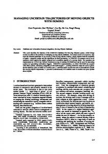
Figure 11(b) shows the result of an experiment with varying Raster networks. The 3D query processing cost remains nearly constant for all networks. This is plausible, since in 3D, we index the trajectories, and the shape of the underlying network is of little influence. However, the 2D cost varies greatly and is for a given query window size lowest for the dataset linked to a network with the lowest number of edges. For small query windows, the 2D cost is generally lower than the 3D query processing cost. With an increased query size, and thus an increased number of transformed query windows, the 2D cost increases over the 3D cost. Again, this break-even point is shifted towards larger query windows for networks with a smaller number of edges. Figure 12 compares the processing of trajectory data (“r2” network) 1000000
100000
IO
IO
10000
r1_2D (144)
r1_3D
r2_2D (544)
r2_3D
r3_2D (2112)
r3_3D
r4_2D (8320)
r4_3D
10000
1000
100 0.25
0.5
1
2
query window extent [%]
(a)
h_2D
h_3D
r2_2D
r2_3D
p_2D
p_3D
4
1000
8
100 0.25
0.5
1
2
4
8
query window extent [%]
(b)
Figure 11: Query performance varying query size: (a) Hilbert, Raster, and Parallel networks and (b) varying Raster networks
The results of the performance study are as follows. Mapping trajectory data to lower dimensions proved beneficial in terms of query processing given the right circumstances! The number of query windows in the 2D case determines its cost and competitiveness to the 3D approach. This number is determined by the density and complexity of underlying road network. The experiments showed that the lower the complexity of a network, the larger a query window could the mapping approach support with a competitive cost. Further, when considering the typical temporal growth of the trajectory data, the 2D approach scales better. The rate of increase of the 2D query processing cost is smaller when compared to the 3D case.
40000 35000 r2_3D
30000
r2_2D
25000 IO
20000 15000 10000 5000 0 75
150
250
time
500
750
5
1000
Figure 12: Query performance varying temporal extent for the Raster network with a varying temporal extent ranging, from 75 to 1000 samples, stemming from 250 moving objects. The size of the query windows (2% spatial extent, 10% temporal extent) was kept constant for all datasets. Both, the 3D and 2D query processing cost is increased for larger datasets. However, the rate of increase for the 3D approach is higher. This overall favors the 2D approach, since trajectory data typically grows with respect to time rather than space (“objects keep on moving, but not necessarily further away”).
4.3
Real Networks
Using real-world networks, we want to confirm the results from the previous section. We additionally want to show the effect of the added cost of query window mapping. Figure 13(a) shows for a varying query size the number of IOs needed in the three- and twodimensional case to process the respective query without considering the mapping cost. At a query size of 0.7%, we reach the break-even point for the San Jose dataset. For the Oldenburg dataset, break-even is at 1.4%. Considering the cost of querying the network in Figure 13(b), the break-even points become 0.4% and 1.1%, respectively. The Oldenburg dataset reaches this break-even point with larger query sizes because of its lower complexity (cf. [15]) and the smaller number of network edges.
100000
IO
IO
oldenburg_2D oldenburg_3D san_jose_2D san_jose_3D
10000
oldenburg_2D oldenburg_3D san_jose_2D san_jose_3D
10000
1000
1000
100 0.25
This work points to several future research directions. One obvious extension is to consider alternative access methods for indexing the trajectory data in the 3D and the 2D spaces. It would be especially interesting to adapt the TB-tree [14] to the 2D data. Another 1000000
1000000
100000
CONCLUSIONS AND FUTURE WORK
Work in the context of spatiotemporal query processing has dealt with the indexing of trajectories by proposing new access methods. This work aims at using off-the-shelf methods for the indexing of trajectories of objects moving in transportation networks. The idea is to exploit the restriction of the data to networks to reduce the dimensionality of the trajectory data. More specifically, this work proposes a mapping approach that exploits that two-dimensional networks can be mapped to one-dimensional intervals. Thus, the dimensionality of trajectories can be reduced from three to two. The important question then becomes the following: given two indices, one for the original 3D data and one for the mapped 2D data, which one is superior in terms of query processing? The mapping of queries to suit the 2D data becomes the critical aspect. In particular, the number of 2D queries that result from the mapping of a 3D query is crucial. The larger it is, the less likely it is that the mapping approach outperforms querying data in the original space. The performance study presents results for varying sets of queries and trajectory data. The data is produced using a network-based generator [2]. Using five different types of networks, three synthetic and two real-world networks, the experiments show that the lower the complexity of a network, the more likely the mapping approach proves to be beneficial over indexing the data in 3D space.
0.5
1 2 query window extent [%]
(a)
4
4
100 0.25
0.5
1 2 query window extent [%]
4
(b)
Figure 13: Query performance varying query size: (a) without and (b) with network query cost
4
extension is to investigate this approach for other types of queries proposed previously [14]. One has to carefully investigate the implications of the mapping approach with respect to indexing in general, e.g., dead space in 3D space vs. 2D space. The trajectory mapping algorithm assumes a Hilbert ordering of the segments. With respect to optimal index structures, more elaborate schemes, such as using the trajectory data for determining the approach for mapping the network edges, might improve the cost of indexing trajectories in 2D space. Also, there are existing approaches to the indexing of moving object data in the 2D case. Comparing them to the performance of the 3D case using R-tree based methods is of interest. Finally, a challenging focus of future work is to apply this method in a practical setting, e.g., using off-the-shelf database technology and applying the presented approach in an application context such as location-based services for mobile devices.
ACKNOWLEDGEMENTS The authors would like to thank Thomas Brinkhoff for providing his network-based data generator as well as for being ever-present with his help and support. We also would like to thank Ouri Wolfson for discussions on this subject during a visit at Aalborg University. This work is supported by the DB-Globe project, funded by the European Commission under contract number IST-2001-32645 and by the Wireless Information Management research training network, funded by the Nordic Academy for Advanced Study.
REFERENCES [1]
[2]
[3]
[4]
[5]
[6]
[7]
[8]
Agarwal, P. K., Arge, L., and Erickson, J.: Indexing Moving Points. In Proc. of the 19th ACM Symposium on Principals of Database Systems, pp.175-186, 2000. Brinkhoff, T.: Generating Network-Based Moving Objects. In Proc. of the 12th Int’l Conference on Scientific and Statistical Database Management, pp. 253-55, 2000. Güting, R.H., Böhlen, M., Erwig, M., Jensen, C.S., Lorentzos, N., Schneider, M., and. Vazirgiannis, M.. A Foundation for Representing and Querying Moving Objects. ACM TODS 25(1):1-42, 2001. Guttman, A.: R-trees: a Dynamic Index Structure for Spatial Searching. In Proc. of ACM-SIGMOD Conference on the Management of Data, pp. 47-57, 1984. Hadjieleftheriou, M., Kollios, G., Tsotras, V., and Gunopulos, D.: Efficient Indexing of Spatiotemporal Objects. In Proc. of the 8th Int’l Conference on Extending Database Technology, pp. 251-268, 2002. Kollios, G., Gunopulos, D., and Tsotras, V., Delis, A., and Hadjieleftheriou, M.: Indexing Animated Objects Using Spatiotemporal Access Methods. IEEE TKDE, 13(5):758777, 2001. Lazaridis, I., Porkaew, K., and Mehrotra, S.: Dynamic Queries Over Mobile Objects. In Proc. of ACM-SIGMOD Conference on the Management of Data, pp. 269-286, 2002. Leutenegger, S., Lopez, M., and Edington, J.: STR: A simple and efficient algorithm for R-tree packing. In Proc. of the 12th Int’l Conference on Data Enginnering, pp. 497–506, 1997.
[9]
Manolopoulos, Y., Theodoridis, Y., and Tsotras, V.: Advanced Database Indexing. Kluwer Academic Publishers, Boston/Dordrecht/London, 2000.
[10] Nascimento, M., Silva, J., and Theodoridis, Y.: Evaluation of Access Structures For Discretely Moving Points. In Proc. of Int’l Workshop on Spatio-Temporal Database Management, pp. 171-188, 1999. [11] Oracle Corporation: Oracle Spatial User’s Guide and Reference, Release 9.2. 2002. [12] Pfoser, D.: Indexing the Trajectories of Moving Objects. IEEE Data Engineering Bulletin, 25(2): 3-9. 2002. [13] Pfoser, D. and Jensen, C.: Capturing the Uncertainty of Moving-Object Representations. In Proc. of the 6th Int’l Symposium on Spatial Databases, pp.111-132, 1999. [14] Pfoser, D., Jensen, C., and Theodoridis, Y.: Novel Approaches to the Indexing of Moving Object Trajectories. In Proc. of the 26th Int’l Conference on Very Large Databases, pp.395-406, 2000. [15] Pfoser, D. and Jensen, C.: Indexing of Network-Constrained Moving Objects. Technical Report, Data and Knowledge Engineering Group, Computer Technology Institute, Greece. http://dke.cti.gr/pubs/tr/pj2003a.pdf, 2003. [16] Pitoura, E., Abiteboul, S., Pfoser, D., Samaras, G., and Vazirgiannis, M.: DB-Globe, A Service-Oriented P2P System for Global Computing. SIGMOD Record, to appear, 2003. [17] Porkaew, K., Lazaridis, I., and Mehrotra, S.: Querying Mobile Objects in Spatio-Temporal Databases. In Proc. of the 7th Int’l Symposium on Advances in Spatial and Temporal Databases, pp. 55-78, 2001. [18] Saltenis, S. and Jensen, C. S.: Indexing of Moving Objects for Location-Based Services. In Proc. of the 18th Int’l Conference on Data Engineering, pp. 463-472, 2002. [19] Saltenis, S., Jensen, C. S., Leutenegger, S., and Lopez, M.: Indexing the Positions of Continuously Moving Objects. In Proc. of ACM-SIGMOD Conference on Management of Data, pp. 331-342, 2000. [20] Sistla, A., Wolfson, O., Chamberlain, S., and Dao, S.: Modeling and Querying Moving Objects. In Proceedings of the 13th International Conference on Data Engineering, pp. 422-432, 1997. [21] Tao, Y. and Papadias, D.: MV3R-Tree: A Spatio-Temporal Access Method for Timestamp and Interval Queries. In Proc. of the 27th Int’l Conference on Very Large Databases, pp. 431-440, 2001. [22] Tayeb, J., Ulusoy, Ö., and Wolfson, O.: A Quadtree-Based Dynamic Attribute Indexing Method. The Computer Journal 41(3), pp. 185-200, 1998. [23] Tzouramanis, T., Vassilakopoulos, M., and Manolopoulos, Y.: Overlapping Linear Quadtrees: A Spatio-Temporal Access Method. In Proceedings of the 6th International Symposium on Advances in Geographic Information Systems, pp. 1-7, 1998.