Indirect Cycle-Time Quantile Estimation for Non-FIFO ... - CiteSeerX

Proceedings of the 2006 Winter Simulation Conference L. F. Perrone, F. P. Wieland, J. Liu, B. G. Lawson, D. M. Nicol, and R. M. Fujimoto, eds.

INDIRECT CYCLE-TIME QUANTILE ESTIMATION FOR NON-FIFO DISPATCHING POLICIES Jennifer McNeill Bekki Gerald T. Mackulak John W. Fowler Industrial Engineering Department Arizona State University Tempe AZ 85287-5906, U.S.A.

system and allow customer delivery dates to be quoted at a level of confidence acceptable to the decision maker. Unfortunately, obtaining estimates of cycle-time quantiles is substantially more difficult than obtaining estimates of the mean cycle-time, and currently available cycle-time quantile estimation techniques have several drawbacks, especially when applied to non-FIFO systems. The most traditional method for obtaining quantile estimates is to use order statistics. This technique requires all observations of the distribution to be stored, resulting in a large data storage requirement. Several techniques have been developed to reduce this data storage burden by modifying the basic order statistics approach (Jain and Chlamtac 1985, Heidelberger and Lewis 1984). However, these approaches generally have the drawbacks of becoming cumbersome to implement when estimates of multiple quantiles are desired and often requiring that the quantiles to be estimated are known in advance. More recently, Chen and Kelton (2006) developed an approach which accommodates estimation of multiple quantiles simultaneously and generates confidence intervals around the estimates, but their approach has the drawback, albeit reduced when compared to order statistics, of requiring significant data storage. The approaches mentioned previously are direct, as they are all obtained by inverting an empirical cumulative distribution function (cdf). As described, these approaches have significant shortcomings. However, they also have the advantage of exhibiting quantile estimation accuracy that is independent of distributional shape. An indirect quantile estimation approach, alternatively, does not build an empirical cdf. Instead, it uses features of the distribution to generate quantile estimates. Indirect techniques have the advantages of requiring low data storage, easily generating estimates of multiple quantiles, and not requiring that the quantiles to be estimated are known in advance. On the other hand, their estimation accuracy is dependent on the shape of the distribution from which quantiles are to be estimated.

ABSTRACT Previous work has shown that the Cornish-Fisher expansion (CFE) can be used successfully in conjunction with discrete event simulation models of manufacturing systems to estimate cycle-time quantiles. However, the accuracy of the approach degrades when non-FIFO dispatching rules are employed for at least one workstation. This paper suggests a modification to the CFE-only approach which utilizes a power data transformation in conjunction with the CFE. An overview of the suggested approach is given, and results of the implemented approach are presented for a model of a non-volatile memory factory. Cycle-time quantiles for this system are estimated using the CFE with and without the data transformation, and results show a significant accuracy improvement in cycle-time quantile estimation when the transformation is used. Additionally, the technique is shown to be easy to implement, to require very low data storage, and to allow easy estimation of the entire cycle-time cumulative distribution function. 1

INTRODUCTION

In today's business environment, with supply-chain complexity increasing, the ability to generate accurate customer delivery dates is crucial. Service-based industries with intricate supply-chains, such as the semiconductor manufacturing industry, compete not only on traditional measures such as cost and product quality, but also on the timely delivery of product to both end-product customers and intermediate parties in the supply-chain. Consequently, the ability to accurately and efficiently estimate customer delivery dates are crucial. Estimates of mean cycle time are often readily available, but using them to generate estimates of delivery dates ignores variability in the cycle time distribution and can result in reduced on-time delivery. Estimates of cycle time quantiles, on the other hand, provide a complete picture of the cycle time distribution for a given

1-4244-0501-7/06/$20.00 ©2006 IEEE

1829

Bekki, Mackulak, and Fowler Yang et al. (2005) suggest such an indirect technique. Their technique uses estimates of the first three moments of the cycle-time distribution to fit a generalized gamma distribution, which is then inverted to obtain cycle-time quantile estimates. An additional advantage of their technique, as opposed to other techniques currently available, both direct and indirect, is that it provides the capability to simultaneously obtain quantile estimates across a range of throughput values, including throughput rates at which simulation runs were not performed. The technique, though, is difficult to implement, and results have only been given for FIFO systems. As non-FIFO dispatching policies are introduced into a system, the cycle-time distribution may change dramatically, making a fit to the generalized gamma distribution inappropriate.

accuracy of the technique can degrade substantially (McNeill et al. 2005b). The CFE was developed to generate quantile estimates from an arbitrary distribution, but it works best for distributions similar to the normal distribution. In manufacturing settings employing FIFO dispatching at all workstations, the cycle time distribution is very close to normal, resulting in high quantile estimation accuracy with the CFE alone. However, as non-FIFO dispatching rules are introduced into the system, the cycle time distribution becomes less and less similar to the normal distribution, and the Cornish-Fisher expansion no longer produces quantile estimates of acceptable quality. This paper suggests a quantile estimation technique specifically appropriate for the cycle time distributions found in manufacturing systems that employ non-FIFO dispatching rules in at least one workstation. The technique combines the CFE with a power data transformation, maintaining the advantages of quantile estimation using the CFE while simultaneously addressing the accuracy issues resulting from non-FIFO dispatching. The remainder of the paper details the approach, and an application of the technique is given for a non-volatile memory factory under basic non-FIFO dispatching policies, both due-date based and non-due date based.

1.1 Quantile Estimation with the Cornish-Fisher Expansion Other previous indirect quantile estimation work (McNeill et al. 2003 and McNeill et al. 2005a) has shown that for manufacturing systems employing FIFO dispatching at all workstations, the Cornish Fisher Expansion (CFE) in conjunction with discrete event simulation provides a cycle time quantile estimation technique which requires low data storage, is easy to implement, has high accuracy, and provides the ability to estimate the entire time cumulative distribution function (cdf) of the cycle-time distribution from a single set of simulation runs. The CFE (Cornish and Fisher 1937) is an infinite expansion that was developed to approximate quantiles of an arbitrary distribution based on the distribution’s moments. When sample moments are used rather than the distribution’s true moments, the CFE can be used to obtain quantile estimates. Equation (1) gives the first four terms of the CFE. In this equation, zα is a quantile from the standard normal distribution, γ1 is the standardized central skewness, γ2 is the standardized central excess kurtosis, σ is the standard deviation, μ is the mean, and Yα is the quantile estimate. To implement the CFE with discrete event simulation models for cycle-time quantile estimation, estimates of the first four moments of the cycle-time distribution are collected during the simulation run at a given throughput rate. These moment estimates are then used with a zα value corresponding to the desired quantile estimate in Equation (1).. xα=zα+1/6(zα2-1)γ1

Yα=μ+σxα, where +1/24(zα3-3zα)γ2-1/36(2zα3-5zα)γ12

2

DATA TRANSFORMATIONS

2.1 Max/Min Data Transformation McNeill et al. (2005b) show that a technique combining a data transformation with the CFE expansion holds promise for improving accuracy in quantile estimation from distributions significantly different from normal. They use the maximum/minimum transformation (Heidelberger and Lewis 1984) with the CFE to estimate quantiles from lognormal distributions, which can have moments similar to distributions found in systems employing non-FIFO dispatching policies. When the max/min transformation is combined with the CFE, desired quantiles are estimated from the transformed distribution using the CFE, after which they transformed back to the original distribution to yield the final quantile estimate. Results showed significant improvement in quantile estimation accuracy when the max/min transformation was used with the CFE, indicating the likelihood that similar improvement would be found when estimating cycle-time quantiles from systems employing non-FIFO dispatching rules in at least one workstation. The maximum/minimum data transformation, however, is a grouping data transformation. It uses more than one data point from the original distribution to yield a single data point in the transformed distribution. As a result of this grouping, data storage requirements are increased, sometimes significantly. Moreover, the size of the group is dependent on the desired quantile estimate; quantile esti-

(1)

McNeill et al., 2005a show that the CFE-based approach yields both precise and accurate estimates for a variety of systems under FIFO dispatching. However, when tested in manufacturing environments employing nonFIFO dispatching policies in at least one workstation, the

1830

Bekki, Mackulak, and Fowler mates closer to the tails of the distribution require larger groups. As a result, estimating multiple quantiles requires the simultaneous maintenance of multiple groups, making the estimation of multiple quantiles difficult. The max/min data transformation, therefore, illustrates that a data transformation has the potential to significantly improve the accuracy of cycle-time quantile estimation with the CFE for extremely non-normal distributions, but it also highlights the need for a non-grouping transformation that can harness the advantages of the CFE-only approach, including very-low data storage and the ability to estimate multiple quantiles easily.

Moreover, although λ=-0.25 is not contained within all four of the confidence intervals, it was a closely competing value for all cases. Table 2: Power Transformations Suggested by Box-Cox for Lognormal Distributions Distribution Lognormal (1, 1.5,1) Lognormal(2,1,2) Lognormal (2,.75,2) Lognormal (3,1,1)

Based on the results shown in Table 2, the CFE in conjunction with the λ=-0.25 power transformation was used to estimate quantiles 0.5, 0.6, 0.7,0.8, 0.9, and 0.99 from a variety of lognormal distributions, including two of the distributions used to select the λ value and 2 not used in its selection. Table 3 shows the results of this experimentation. Theoretical quantiles for the examined distributions are known, so the results in Table 3 show the relative percent difference between the quantiles estimated using the CFE with the power (-.25) transformation and their theoretical counterparts. To generate the results, Minitab was used to randomly generate 500,000 independent random observations from each distribution. Each observation was then transformed using the power (-.25) transformation, and the sample moments of the transformed observations were calculated. The CFE was then used to estimate quantiles, and the quantile estimates were then transformed back to their original distribution. For all the investigated distributions, estimates of quantiles less than or equal to 0.9 are very accurate. The accuracy declines in some cases as the quantile estimated tends toward the extreme tail, but that is not unexpected, as quantiles from the tails are significantly more difficult to estimate. In summary, the results given in Table 3 demonstrates that a quantile estimation technique combining the power (-.25) transformation with the CFE has the potential to generate accurate quantile estimates from a variety of distributions similar to those found in models of manufacturing systems employing non-FIFO dispatching.

2.2 Power Transformations The power family of transformations xλ, where λ is a parameter to be determined, is a non-grouping a transformation commonly used to correct for non-normality (Montgomery et al. 2001). Since the CFE is known to estimate quantiles more accurately for distributions more similar to the normal distribution, a normalizing power transformation is a reasonable option for combining with the CFE. To implement a power transformation with the CFE to estimate cycle-time quantiles, each individual data point, x, is simply raised to the power λ before the moment estimates are made. The moment (and subsequent quantile) estimates are then made from the transformed distribution, and the quantile estimates are then transformed back to their original distribution to give the final cycle-time quantile estimate. To determine which transformation from the family of power transformations to use, a variety of log-normal distributions were examined. These distributions were used since their first four moments are similar to those seen in cycle-time distributions. Table 1 shows the distributional parameters as well as their first four moments. The. parameters, in order of their listing, are: location parameter, scale parameter, and threshold parameter. Table 1: Lognormal Distribution Moments Distribution Lognormal (1, 1.5,1) Lognormal(2,1,2) Lognormal (2,.75,2) Lognormal (3,1,1)

Mean 9.400 14.291 11.661 34.002

Optimal Lambda (-.382 - .346) (-.316,-.273) (-.294, -.234) (-.086, -.054)

Variance Skewness Kurtosis 706.620 26.690 1314.890 271.025 6.540 102.030 62.393 2.660 12.500 1915.509 6.000 71.300

Table 3: Accuracy of Quantile Estimation for Selected Lognormal Distributions when the CFE is Combined with a Power (-.25) Transformation Quantile

For each of the lognormal distributions investigated, Minitab was used to generate 500,000 random data points and then to perform the Box-Cox transformation on the random data. Table 2 shows the result of these calculations. The second column of Table 2 gives a 95% confidence interval on the suggested λ value for the power transformation. In all examined cases, a negative power transformation is optimal. Also, the average value of the optimal lambda values across all four cases is λ=-0.25.

0.5 0.6 0.7 0.8 0.9 0.99

1831

Lognormal (0,1,0) 1.31% 1.04% 0.52% -0.35% -1.92% -5.32%

Lognormal (1, .75, 1) 0.18% -0.07% -0.33% -0.58% -0.73% -0.43%

Lognormal (3,1,1) -1.30% -1.02% -0.38% 0.69% 2.38% 0.42%

Lognormal (1,1.5,1) 2.14% -0.04% -2.27% -3.94% -3.38% 14.19%

Bekki, Mackulak, and Fowler 3

rework. To run the model, the Factory Explorer software(Chance 1995) was used. The system was examined under the following dispatching rules: last in first out (LIFO), random (RAND), earliest due date first (EDD), and critical ratio (CR). The EDD and CR dispatching rules are both due-date based, while LIFO and RAND are not. For the due-date based rules, due dates were assigned by giving an offset based on the raw processing time (RPT) of each job. Equation (2) shows the specific method in which due dates for each job were assigned. Also, the form of the CR rule used in this experimentation is given in Equation (3), where DD is the due date, TNOW is the current simulation time, and TRPT is the total remaining processing time. A variety of forms of the CR dispatching rule exist; this version was chosen as it was found to give better performance than its alternatives (Rose 2002).

CYCLE-TIME QUANTILE ESTIMATION PROCEDURE

The following procedure combining the CFE with the power (-.25) transformation was implemented to obtain the experimental results given in the remainder of the paper. High level steps for the procedure are given below, and it is assumed that users of the procedure will use an appropriate number of replications, appropriate run-length, and will take steps to avoid bias in the estimates due to the warm-up period of each simulation run. 1.

2.

For each simulation replication (a) Run simulation replication and transform each cycle-time observation, x, to be 4 x t = 1 x . From the distribution of xt values, calculate an estimate of the sample mean an estimate of the sample standard deviation, an estimate of the sample central, standardized skewness, and an estimate of the sample central, standardized, excess kurtosis. (b) Estimate the (1 - α) quantile of the transformed distribution, where α is the desired quantile estimate from the original cycle-time distribution, using the first four terms of the CFE given in Equation (1). (c) Transform the cycle-time quantile estimate back to the original distribution by raising the estimate from the transformed distribution to the fourth power and taking the inverse. Calculate the mean cycle-time quantile estimate as the mean of all the cycle-time quantile estimates obtained during all simulation runs.

(2)

⎧1 + DD − TNOW if DD > TNOW 1 + TRPT ⎪ CR = ⎨ 1 otherwise ⎪ ( (1+TNOW-DD ) * (1 + TRPT ) ) ⎩

(3)

Also, since theoretical quantiles are unknown for the system, direct estimates using order statistics were obtained for the system. To obtain direct estimates, ten replications of 30 years each were run. For each replication, the 0.01, 0.1, 0.2, 0.3, …, 0.8, 0.9, 0.99 cycle-time quantiles were estimated. For each quantile, the average value across all ten replications was taken as the final estimate. These values were considered to be the “true” cycle-time quantiles from the system and were used for comparison with indirectly estimated values.

Notice that because the power(-.25) transformation is an inverse transformation, the (1-α) quantile of the transformed distribution must be estimated to obtain an estimate of the α quantile from the original distribution. 4

due _ date = creation _ time + EXP (10 * RPT )

4.1 Experimental Results Table 3 summarizes the results across all the explored dispatching policies when the system was simulated at 95% throughput rate. Since the dispatching policies have greater and greater impact on the cycle-time distribution as the throughput rate gets closer and closer to 100%, the results shown in Table 1 represents a “worst-case” scenario in which the cycle-time distribution is extremely different than it would be under its FIFO counterpart. In Table 3, the average deviation column represents the average relative percentage difference from the directly estimated values across all the estimated cycle-time quantiles (0.01, 0.1, 0.2, 0.3, …, 0.8, 0.9, .99). The maximum deviation column gives the largest deviation among all estimated quantiles, and the final column of the table shows which cycle-time quantile corresponds to the maximum deviation. Table 3 demonstrates that for all distributions examined, the combination of the power (-.25) transformation with the CFE yields cycle-time quantile estimates with

EXPERIMENTATION AND RESULTS

To assess the accuracy of using the power (-.25) transformation in conjunction with the CFE for estimating cycletime quantiles in realistically sized systems, a model of a non-volatile memory factory was used. The model is a slight modification to Testbed Data Set #1 from the Modeling and Analysis of Semiconductor Manufacturing (MASM) lab at Arizona State University, which can be obtained at . The model has two products, 83 tool groups, and 15 process steps per mask layer. It utilizes non-FIFO dispatching at all workstations and also accounts for operators, machine breakdown, preventive maintenance, and product

1832

Bekki, Mackulak, and Fowler high accuracy. The LIFO dispatching rule generated the cycle-time distribution which was the most difficult from which to estimate quantiles. However, even for the LIFO distribution, the cycle-time quantile estimates are still extremely close to the directly estimated values. The maximum percentage deviation was only 4.08%, and the average percent deviation was less than 0.5%.

Figure 2 gives similar results to Figure 1, but for the due-date based rule, EDD. Also, Figure 2 shows results for the system at 60% throughput rate. For this system, the 60% throughput rate is interesting because of batching. As the throughput rate gets lower, jobs wait longer for batches to form, and the impact on the cycle time distribution becomes greater. Figure 2 illustrates that the quantile estimates obtained using the data transformation (the line marked with squares) are significantly more accurate than those obtained with the CFE alone. In fact, estimates using the CFE alone (the line marked with circles in Figure 2) are up to 150% different from the directly estimated values. Finally, Figure 3 gives a feel for how the throughput rate of the system impacts the accuracy of the cycle-time quantile estimates obtained with the CFE in conjunction with the power (-.25) data transformation. The x-axis of Figure 3 shows the throughput rate, while the y-axis again gives the relative percent difference between directly and indirectly estimated cycle-time quantiles for the system under LIFO dispatching. Each line in Figure 3 represents a different quantile; the 0.5, 0.7, 0.9, and 0.99 quantiles are shown. All the cycle-time quantile estimates were obtained using the CFE in conjunction with the power (-.25) data transformation. Figure 3 shows that the estimate of the 0.99 quantile at a 60% throughput rate is approximately 9% different from the direct estimate. Although this estimate is less precise than the other presented results, it is likely explained by the fact that quantiles in the extreme tails, like the 0.99 quantile, are more difficult to estimate. Additionally, at a 60% throughput rate, batching, in addition to the dispatching policy, is influencing the cycle time distribution, making indirect cycle-time quantile estimation even more difficult.

Table 3: Quantile Estimation Accuracy at 0.95 Traffic Intensity for Non-Volatile Memory Factory Lab Dispatching Policy Average Deviation Maximum Devation Quantile RAND -0.003% -0.687% 0.01 LIFO 0.229% -4.083% 0.90 EDD -0.019% -0.658% 0.01 CR -0.045% -0.532% 0.01

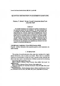
Figure 1 shows the impact of the power (-.25) transformation with the CFE on the accuracy of cycle-time quantile estimates when the system is simulated at 95% throughput rate. The x-axis of Figure 1 shows the quantile being estimated, while the y-axis gives the relative percentage difference from the directly estimated values. The line marked with squares shows the quantile estimates obtained using the CFE without a data transformation, while the line marked with circles shows the percentage difference for the same quantile estimates when the power (-.25) data transformation is combined with the CFE. Clearly, combining the CFE with the data transformation results in a significant improvement in accuracy for this system. Cycle-time quantile estimates obtained without the data transformation are up to 50% off, while estimates obtained using the data transformation are no more than 4.1% different than the directly estimated values. 60.000%

150.000%

40.000%

100.000%

30.000% 20.000%

Relative Percent Error

Relative Percent Error

50.000%

10.000% -

0.000% -10.000% -20.000% -30.000%

50.000% 0.000% -50.000% -100.000% -150.000%

0

0.2

0.4

0.6

0.8

1

Quantile Estimated Non-Transformed Data

-200.000%

0

Transformed Data

0.2

0.4

0.6

0.8

1

Quantile Estimated

Figure 1: Relative Percent Difference Between CycleTime Quantiles Estimated Using the CFE with the Power (-0.25) Data Transformation and Quantiles Estimated Directly Using Order Statistics for the Non-Volatile Memory Factory Under LIFO Dispatching at a Throughput Rate of 95%

60 TI Non-Transformed Data

60TI Transformed Data

Figure 2: Relative Percent Difference Between the CycleTime Quantiles Estimated Using the CFE with the Power (-.25) Data Transformation and Quantiles Estimated Directly Using Order Statistics for the Non-Volatile Memory Factory Under EDD Dispatching at a Throughput Rate of 60%

1833

Bekki, Mackulak, and Fowler Detailed results were also collected for EDD and CR policies. The outcomes were comparable to those shown in Figures 1 – 3 for the LIFO and EDD policies and were left out for the sake of brevity.

Lastly, attention could be given to combining the work of Yang et al. (2005) with the CFE-based approach discussed in this paper. The combination of these techniques would yield a powerful cycle-time quantile estimation technique. It would capture the significant benefit of the Yang et al. approach, which gives quantile estimation capability at multiple throughput rates simultaneously, while also harnessing the ease of implementation and robustness to a variety of cycle-time distributions that the CFE-based approach includes.

10.000%

Relative Percent Error

8.000% 6.000% 4.000% 2.000%

ACKNOWLEDGMENTS

0.000%

This research has been supported in part by grant P011335 from the Factory Operations Research Center (FORCe) that is jointly funded by the Semiconductor Research Corporation (SRC) and by International SEMATECH and in part by a doctoral fellowship sponsored by Intel Corporation and SRC.

-2.000% -4.000% -6.000% 0.6

0.7

0.8

0.9

1

System Traffic Intensity 0.5 Quantile

0.7 Quantile

0.9 Quantile

0.99 Quantile

Figure 3: Relative Percent Difference Between Selected Cycle-Time Quantiles (0.5, 0.7, 0.9, and 0.99) of the NonVolatile Memory Factory Under LIFO Dispatching Estimated Using the CFE with the Power (-.25) Transformation and Those Estimated Directly Using Order Statistics as a Function of the System Throughput Rate 5

REFERENCES Chance, F. 1995. Factory explorer, integrated capacity, cost, and cycle-time analysis, version2, level 2, beta 2, user’s guide and reference. Dublin, California: Wright Williams & Kelly. Chen, E.J., and W.D. Kelton. 2006. Quantile and toleranceinterval estimation in simulation. European Journal of Operational Research 168: 520-540. Cornish, E.A., and R.A. Fisher. 1937. Moments and cumulants in the specification of distributions. Revue de l'Institut International de Statistique 5: 307-320. Heidelberger, P.m and P. Lewis. 1984. Quantile estimation in dependent sequences. Operations Research 32: 185-209. Jain, R., and I. Chlamtac. 1985. The P2 algorithm for dynamic calculation of quantiles and histograms without storing observations. Communications of the ACM 28: 1076-1085. McNeill, J., G. Mackulak, and J. Fowler. 2003. Indirect estimation of cycle time quantiles from discrete event simulation models using the Cornish-Fisher expansion, In Proceedings of the 2003 Winter Simulation Conference, ed. S. Chick, P. J. Sánchez, D. Ferrin, and D. J. Morrice, 1377 – 1382. McNeill, J., G. Mackulak, J. Fowler, and B. Nelson. 2005a. Indirect cycle time quantile estimation using the Cornish-Fisher expansion. In review at IIE Transactions. Available as paper ASU-IE-ORPS-2004-001 via . McNeill, J., B. Nelson, B., J. Fowler, and G. Mackulak. 2005b. Cycle Time quantile estimation in systems employing dispatching rules. In Proceedings of the 2005 Winter Simulation Conference, ed. M. E. Kuhl,

DISCUSSION AND FUTURE WORK

The results presented in this paper illustrate that the nongrouping power(-.25) transformation can be successfully used in conjunction with the CFE to estimate cycle-time quantiles in systems employing non-FIFO dispatching rules. The technique maintains the primary benefits of the CFE – only approach while simultaneously addressing its accuracy issues. For a variety of simple dispatching rules common to manufacturing systems, experimentation on a realistically sized model showed that the procedure produces accurate cycle-time quantile estimates across a wide range of quantiles. Additionally, the technique requires the storage of only four data points, used to calculate sample moment estimates, is easy to implement, and it does not require the quantiles for which estimates are desired to be known in advance. Moreover, after the sample moments are known, a discrete estimate of the entire cdf of the cycle-time distribution can be obtained by simply changing the zα value in Equation 1. Future work in this area will include more exhaustive testing of the procedure on queueing systems of different topographies. Additionally, due date assignment policies that have tighter due dates will be examined, including policies that force some jobs to be late as soon as they are created. Experimentation in this paper is limited to a single system, and further testing the robustness of the technique on cycle-time distributions of additional shapes will add to its credibility.

1834

Bekki, Mackulak, and Fowler N. M. Steiger, F. B. Armstrong, and J. A. Joines, 751755. Montgomtery, D.C., E.A. Peck., and G.G. Vining. 2001. Introduction to linear regression analysis, third edition. New York: John Wiley & Sons, Inc. Rose, O. 2002. Some issues of the critical ratio dispatch rule in semiconductor manufacturing. In Proceedings of the 2002 Winter Simulation Conference, ed. E. Yücesan, C.H. Chen, J.L. Snowdon, and J.M. Charnes, 1401 – 1405. Yang, F., B.E. Ankenman, B.E. and B.L. Nelson. 2005. Estimation of percentiles of cycle time in manufacturing simulation. In Proceedings of the 2005 Winter Simulation Conference, ed. M. E. Kuhl, N. M. Steiger, F. B. Armstrong, and J. A. Joines, 475-484.. AUTHOR BIOGRAPHIES JENNIFER M. BEKKI is a Ph.D. candidate in the Industrial Engineering department at Arizona State University. Her research interests are in discrete-event simulation methodology and manufacturing applications in the semiconductor industry. Prior to beginning her Ph.D. studies, she served as an intern in the Operational Decision Support Technologies group at Intel, and she is currently funded on an SRC/Intel Doctoral Fellowship. Her email address is . GERALD T. MACKULAK is an Associate Professor of Engineering in the Department of Industrial Engineering at Arizona State University. He is a graduate of Purdue University receiving his B.Sc., M.Sc., and Ph.D. degrees in the area of Industrial Engineering. His primary area of research is simulation applications within manufacturing with a special focus on automated material handling within semiconductor manufacturing. His email address is . JOHN W. FOWLER is a Professor of Industrial Engineering at Arizona State University (ASU) and is the Center Director for the Factory Operations Research Center that is jointly funded by International SEMATECH and the Semiconductor Research Corporation. His research interests include modeling, analysis, and control of semiconductor manufacturing systems. Dr. Fowler is a member of ASEE, IIE, INFORMS, POMS, and SCS. He is an Area Editor for SIMULATION: Transactions of the Society for Modeling and Simulation International and an Associate Editor of IEEE Transactions on Electronics Packaging Manufacturing. He is an IIE Fellow and is on the Winter Simulation Conference Board of Directors. His email address is .

1835