function is found by taking the inverse Fourier transform of the PSD. ...... locations from stereo images of points in a
INFERENCE AND UPDATING OF PROBABILISTIC STRUCTURAL LIFE PREDICTION MODELS
A Thesis Presented to The Academic Faculty by Richard J. Cross
In Partial Fulfillment of the Requirements for the Degree Doctor of Philosophy in the Department of Aerospace Engineering
Georgia Institute of Technology December 2007
INFERENCE AND UPDATING OF PROBABILISTIC STRUCTURAL LIFE PREDICTION MODELS
Approved by: Professor Andrew Makeev, Advisor Department of Aerospace Engineering Georgia Institute of Technology
Professor George Kardomateas Department of Aerospace Engineering Georgia Institute of Technology
Professor Erian Armanios Department of Aerospace Engineering Georgia Institute of Technology
Dr. Jack Zhao Technical Leader, Structural Methods and Prognostics Sikorsky Aircraft Corporation
Professor Bruce Ellingwood Department of Civil and Environmental Engineering Georgia Institute of Technology
Date Approved: September 21, 2007
ACKNOWLEDGEMENTS
I first thank my academic advisor Dr. Andrew Makeev for providing important guidance while granting me the freedom to explore and implement new ideas. His support and trust were vital to the completion of this work. Working with Dr. Makeev has been an invaluable learning experience and given me confidence in my work and myself. I am grateful to Dr. Erian Armanios for his mentoring through my time at Georgia Tech and his service on my committee. His unique and brilliant way of thinking has been influential to me. I am also thankful for the many opportunities that he has given me during my time at Georgia Tech. Thanks go to Dr. Bruce Ellingwood for inspiring teaching, serving on my committee, and providing a wealth of knowledge relevant to this thesis. I am privileged to have the chance to learn from a researcher of such caliber and reputation. I would also like to thank Dr. George Kardomateas and Dr. Jack Zhao for their time and assistance as members of my thesis committee. I thank Dr. Zhao for his collaboration on portions of this research, as well. I wish to acknowledge funding for portions of this work from the Center for Rotorcraft Innovation and the Georgia Institute of Technology Vertical Lift Research Center of Excellence. I am also grateful to Terry Larchuk of The Boeing Company, Jeff Schaff of Sikorsky Aircraft Corporation, and Dr. Jim Newman of Mississippi State University for their collaboration on several of the tasks that were performed in this research. I wish to thank my classmates for helping me enjoy my graduate studies. In particular, I thank Dr. Stefano Gonella and Derek Reding for being great friends
iii
from the time I enrolled at Georgia Tech. I am also thankful for my lab mates Xinyuan Tan, Yihong He, Samer Tawfik, Dr. Serkan Ozbay, Dr. Roxanna Vasilescu, Christopher Ignatius, and Robert Haynes. I thank my parents Dr. John Cross and Dr. Virginia Cross for their love and support. They are my role models, and I try every day to make them proud. I also thank my brothers Robert and David Cross for their friendship, especially during my graduate work. I am very fortunate that we were all able to study together on the same campus. Most importantly, I am grateful to my wife and best friend Christiane Gumera. Her love and the happiness she brings to my life gives me the strength to work hard and reach for my goals.
iv
TABLE OF CONTENTS ACKNOWLEDGEMENTS . . . . . . . . . . . . . . . . . . . . . . . . . . . .
iii
LIST OF TABLES . . . . . . . . . . . . . . . . . . . . . . . . . . . . . . . . .
viii
LIST OF FIGURES . . . . . . . . . . . . . . . . . . . . . . . . . . . . . . . .
ix
SUMMARY . . . . . . . . . . . . . . . . . . . . . . . . . . . . . . . . . . . . .
xi
I
INTRODUCTION . . . . . . . . . . . . . . . . . . . . . . . . . . . . . .
1
1.1 Motivation . . . . . . . . . . . . . . . . . . . . . . . . . . . . . . .
1
1.1.1
Dynamic and Airframe Components . . . . . . . . . . . . .
1
1.1.2
Flaw-Tolerant and Damage-Tolerant Design . . . . . . . . .
3
1.1.3
Economic Drivers . . . . . . . . . . . . . . . . . . . . . . . .
4
1.2 Condition Based Maintenance . . . . . . . . . . . . . . . . . . . . .
4
1.2.1
Probabilistic Modeling and Condition Based Maintenance .
5
1.2.2
Stochastic Updating . . . . . . . . . . . . . . . . . . . . . .
6
1.3 Scope and Objectives II
. . . . . . . . . . . . . . . . . . . . . . . . .
7
BACKGROUND . . . . . . . . . . . . . . . . . . . . . . . . . . . . . . .
9
2.1 Structural Component Life Prediction . . . . . . . . . . . . . . . .
9
2.1.1
Safe Life Methods . . . . . . . . . . . . . . . . . . . . . . .
9
2.1.2
Fracture Mechanics . . . . . . . . . . . . . . . . . . . . . . .
11
2.1.3
Spectrum Loading . . . . . . . . . . . . . . . . . . . . . . .
14
2.2 Probabilistic Modeling of Fatigue . . . . . . . . . . . . . . . . . . .
15
2.2.1
Probabilistic Safe-Life Models . . . . . . . . . . . . . . . . .
15
2.2.2
Probabilistic Fracture Mechanics Models . . . . . . . . . . .
16
2.3 Inference of Probabilistic Failure Models . . . . . . . . . . . . . . .
21
2.3.1
Random Variable Model Inference . . . . . . . . . . . . . .
21
2.3.2
Random Process Model Inference . . . . . . . . . . . . . . .
22
2.4 Bayesian Inference and Updating of Failure Models . . . . . . . . .
23
v
III
BAYESIAN FORMULATION . . . . . . . . . . . . . . . . . . . . . . . .
26
3.1 Hierarchical Bayesian Updating Formulation . . . . . . . . . . . . .
26
3.1.1
Likelihood Function Determination . . . . . . . . . . . . . .
28
3.1.2
Prior Distribution Specification . . . . . . . . . . . . . . . .
29
3.1.3
Hyperprior Distribution Specification . . . . . . . . . . . . .
30
3.2 Posterior Simulation Schemes . . . . . . . . . . . . . . . . . . . . .
31
3.2.1
Rejection Sampling . . . . . . . . . . . . . . . . . . . . . . .
31
3.2.2
Markov Chain Monte Carlo . . . . . . . . . . . . . . . . . .
33
3.2.3
The Gibbs Sampler . . . . . . . . . . . . . . . . . . . . . . .
35
3.3 Simplified Hyperparameter Updating . . . . . . . . . . . . . . . . .
39
UPDATING OF HIGH-CYCLE SAFE-LIFE MODELS . . . . . . . . . .
41
4.1 Description of Input Data . . . . . . . . . . . . . . . . . . . . . . .
41
4.2 Bayesian Model Construction . . . . . . . . . . . . . . . . . . . . .
44
4.3 Posterior Simulation . . . . . . . . . . . . . . . . . . . . . . . . . .
46
4.4 Simulation Results . . . . . . . . . . . . . . . . . . . . . . . . . . .
47
EQUIVALENT INITIAL FLAW SIZE INFERENCE . . . . . . . . . . .
53
5.1 Description of Input Data . . . . . . . . . . . . . . . . . . . . . . .
53
5.2 Bayesian Model Construction . . . . . . . . . . . . . . . . . . . . .
53
5.3 Posterior Simulation . . . . . . . . . . . . . . . . . . . . . . . . . .
56
5.4 Simulation Results . . . . . . . . . . . . . . . . . . . . . . . . . . .
57
5.5 Updating Fleet-Level Parameters . . . . . . . . . . . . . . . . . . .
61
5.6 Updating Residual Life Distribution . . . . . . . . . . . . . . . . .
63
HIERARCHICAL GROWTH RATE MODELING . . . . . . . . . . . .
67
6.1 Description on Input Data . . . . . . . . . . . . . . . . . . . . . . .
67
6.2 Bayesian Model Construction . . . . . . . . . . . . . . . . . . . . .
67
6.3 Posterior Simulation . . . . . . . . . . . . . . . . . . . . . . . . . .
72
6.4 Simulation Results . . . . . . . . . . . . . . . . . . . . . . . . . . .
73
VII CONCLUSIONS . . . . . . . . . . . . . . . . . . . . . . . . . . . . . . .
82
IV
V
VI
vi
VIII FUTURE WORK . . . . . . . . . . . . . . . . . . . . . . . . . . . . . .
84
8.1 Advanced Measurement and Inspection Techniques . . . . . . . . .
84
8.1.1
Accurate Damage/Defect Strain Measurement . . . . . . . .
84
8.1.2
Residual Stress Measurement . . . . . . . . . . . . . . . . .
85
8.2 Analytical Capabilities . . . . . . . . . . . . . . . . . . . . . . . . .
85
8.2.1
Random Process Models . . . . . . . . . . . . . . . . . . . .
85
8.2.2
Loads Variability . . . . . . . . . . . . . . . . . . . . . . . .
85
8.3 Experimental Verification . . . . . . . . . . . . . . . . . . . . . . .
86
8.3.1
Verification of Probabilistic Crack Growth Models
. . . . .
86
8.3.2
Application to Full-Scale Components . . . . . . . . . . . .
86
REFERENCES . . . . . . . . . . . . . . . . . . . . . . . . . . . . . . . . . . .
87
VITA . . . . . . . . . . . . . . . . . . . . . . . . . . . . . . . . . . . . . . . .
94
vii
LIST OF TABLES 1
Normalized high-cycle spectrum for helicopter dynamic component . .
42
2
Maintenance data crack and corrosion findings . . . . . . . . . . . . .
43
3
Probabilities of crack initiation for at-risk components . . . . . . . . .
48
4
Probabilities of crack initiation for at-risk components . . . . . . . . .
50
5
Comparison of posterior statistics for distribution parameters . . . . .
59
6
Equivalent initial flaw size statistics comparison . . . . . . . . . . . .
60
7
Data description for AISI 4340 short-crack tests [65] . . . . . . . . . .
68
8
Point estimates of hyperparameters from pooled-data regressions . . .
70
9
Numerical values for generalized linear model hyperprior parameters .
71
10
Posterior AISI 4340 short-crack growth parameter statistics . . . . . .
77
11
Posterior predictive AISI 4340 short-crack growth parameter statistics
79
viii
LIST OF FIGURES 1
Comparison of dynamic and airframe component crack growth . . . .
2
2
Typical crack velocity - stress intensity range relationship . . . . . . .
12
3
Virkler data set [69] . . . . . . . . . . . . . . . . . . . . . . . . . . . .
19
4
Virkler crack velocity data [69] . . . . . . . . . . . . . . . . . . . . . .
19
5
Updated and prior density functions for median endurance limit . . .
48
6
Updated and prior distribution functions for median endurance limit
49
7
Posterior and prior predictive density functions for endurance limit, E∞ 51
8
Updated life distribution for uninspected components . . . . . . . . .
52
9
Double corner crack from lap joint rivet hole . . . . . . . . . . . . . .
54
10
Simulated lap joint crack inspection data set . . . . . . . . . . . . . .
54
11
Marginal posterior distribution for Weibull shape parameter . . . . .
58
12
Marginal posterior distribution for Weibull scale parameter . . . . . .
58
13
Marginal posterior distribution for growth rate standard deviation . .
59
14
Posterior predictive equivalent initial flaw size distribution . . . . . .
60
15
Posterior predictive distribution for crack growth history . . . . . . .
61
16
Probability of detection curve . . . . . . . . . . . . . . . . . . . . . .
62
17
Updated distribution of remaining life . . . . . . . . . . . . . . . . . .
65
18
Detail on updated distribution of remaining life . . . . . . . . . . . .
65
19
Crack growth rate data for AISI 4340 steel . . . . . . . . . . . . . . .
68
20
Autocorrelations from Gibbs simulation . . . . . . . . . . . . . . . . .
73
21
Marginal posterior densities of mean regression intercepts . . . . . . .
74
22
Marginal posterior densities of mean regression slopes . . . . . . . . .
74
23
Marginal posterior densities of regression intercept variances . . . . .
75
24
Marginal posterior densities of regression slope variances . . . . . . .
75
25
Marginal posterior densities of regression error variances . . . . . . .
76
26
Posterior predictive densities of regression intercepts . . . . . . . . . .
78
27
Posterior predictive densities of regression slopes . . . . . . . . . . . .
78
ix
28
Comparison of growth rate predictions to data at R = 0.5 . . . . . .
80
29
Comparison of growth rate predictions to data at R = 0.0 . . . . . .
80
30
Comparison of growth rate predictions to data at R = -1.0 . . . . . .
81
x
SUMMARY
Aerospace design requirements mandate acceptable levels of structural failure risk. Probabilistic fatigue models enable estimation of the likelihood of fatigue failure. A key step in the development of these models is the accurate inference of the probability distributions for dominant parameters. Since data sets for these inferences are of limited size, the fatigue model parameter distributions are themselves uncertain. A hierarchical Bayesian approach is adopted to account for the uncertainties in both the parameters and their distribution. Variables specifying the distribution of the fatigue model parameters are cast as hyperparameters whose uncertainty is modeled with a hyperprior distribution. Bayes’ rule is used to determine the posterior hyperparameter distribution, given available data, thus specifying the probabilistic model. The Bayesian formulation provides an additional advantage by allowing the posterior distribution to be updated as new data becomes available through inspections. By updating the probabilistic model, uncertainty in the hyperparameters can be reduced, and the appropriate level of conservatism can be achieved. In this work, techniques for Bayesian inference and updating of probabilistic fatigue models for metallic components are developed. Both safe-life and damagetolerant methods are considered. Uncertainty in damage rates, crack growth behavior, damage, and initial flaws are quantified. Efficient computational techniques are developed to perform the inference and updating analyses. The developed capabilities are demonstrated through a series of case studies.
xi
CHAPTER I
INTRODUCTION 1.1
Motivation
Practical engineering materials and structures contain defects and cracks. Cyclic loading can cause defects to nucleate cracks and existing cracks to propagate through fatigue processes. The initiation and growth of fatigue cracks may lead to the failure of structural components at loads below design levels, limiting their useful life. Thus fatigue considerations must be addressed if the ability of a structure to withstand design loads is to be ensured for the duration of its specified life. Fatigue risk is especially acute for rotorcraft, where vibratory loads are significant, and structural failures often result in fatalities and loss of expensive equipment. Assessments of the probability of a fatigue failure and its consequences are required to quantify the fatigue risk of a structure properly. Evaluating the consequences of a fatigue failure, whether catastrophic or benign, is fairly straightforward and can be done using established methods of structural analysis. Methods for accurately estimating the likelihood of fatigue failure without costly replicated full-scale testing are less developed, however. 1.1.1
Dynamic and Airframe Components
Rotorcraft parts can be divided into two basic groups based on their cyclic loading environment: dynamic components and airframe components. Dynamic components are subjected to high-frequency, low-amplitude loading during all operations of the aircraft, and examples include shafts, powerplant and drivetrain components, and rotor head components. The load spectra of airframe components are dominated by higher-amplitude, non-vibratory loads, such as ground-air-ground cycles. The 1
Crack Length
Dynamic Component Airframe Component
Detectable Crack Length
Time in Service
Figure 1: Comparison of dynamic and airframe component crack growth difference in the fatigue loading environment between the two groups results in two different regimes of fatigue damage accumulation. The useful lifetime of a dynamic component is dominated by the crack initiation process, whereas crack propagation occupies a larger part of an airframe component’s lifetime. This distinction between crack growth histories of dynamic and airframe components is depicted schematically in Figure 1. Typically, dynamic components are designed so that no detectable fatigue cracks initiate during a pre-determined service life. The part is replaced when damage, such as a gouge, dent, or corrosion pit of a specified size has been found or the predetermined life limit has been reached. The damage size criteria for replacement are usually blanket specifications that do not consider the specific geometry and location of the flaw. In many cases these limits are historical and have not been substantiated with either analysis or experiment. Without an analysis of the actual flaw,
2
serviceable limits must be set by assuming worst-case conditions, and are necessarily over-conservative. Likewise, service life limits prescribed for each component are generally over-conservative since they are determined assuming worst-case conditions instead of actual conditions, as well. Thus many components may be retired with significant useful life remaining due to exceeding either damage or life limits. Retirement lifetimes are generally not specified for inspectable airframe components. Rather, a maintenance schedule is specified in advance such that cracks below a certain size will not reach a critical length between inspections. Worst-case loading and material properties are usually assumed when determining inspection intervals leading to an over-conservative inspection schedule. 1.1.2
Flaw-Tolerant and Damage-Tolerant Design
Updated federal government helicopter certification regulations require that fatigue life substantiation include consideration of possible flaws or damage present in critical locations of structures [1]. The flaw-tolerant approach has been used successfully to comply with the new requirement for the certification of Sikorsky S-92 dynamic components [2]. In this approach, fatigue life testing is performed with a representative flaw located at the most critical location of the part. Component replacement times and inspection intervals are specified based on experimentally determined fatigue lives in the presence of barely detectable flaws and clearly detectable flaws, respectively [68]. For airframe components where the crack propagation time is the dominant portion of the fatigue life, damage tolerance analysis (DTA) has been used successfully to establish retirement times and inspection intervals. DTA is used to demonstrate the ability of the structure to maintain a specified residual strength for a certain period of use after sustaining damage [68]. Such an analysis requires characterization of inherent flaws, crack growth behavior, non-destructive inspection (NDI) methods, loads,
3
and service damage [9]. These data are used as inputs to a physics-based based life prediction model to establish the residual strength and the reliability as a function of continued usage. 1.1.3
Economic Drivers
Accounting for fatigue life uncertainty with conservative blanket maintenance practices ensures some level of reliability but does so in an economically inefficient manner. By achieving the proper level of conservatism, savings may be realized in direct maintenance costs in addition to improving rotorcraft fleet utilization. In the particular case of the US Army helicopter fleet, fatigue-critical parts only serve an average of roughly 25% of their design life before replacement under the current damage allowables [74]. Thus the parts cost alone is about 300% larger than the design maintenance replacement cost. In addition, the rotorcraft spend up to four times more hours in maintenance than designed, necessitating a larger fleet to achieve operational requirements. White and Vaughan show that increasing the average replacement interval from 25% to 33% of the design life limit should result in downtime and replacement cost reductions of approximately 25% [74]. Additional utilization benefits may be achieved through flexibility in inspection intervals. By lengthening intervals, some component inspections may be combined into the same maintenance action or removed altogether.
1.2
Condition Based Maintenance
Condition Based Maintenance (CBM) attempts to improve cost-efficiency and fleet utilization by scheduling inspections, repairs, and retirement for a single component based on its own unique service history, maintenance, and inspection record [46]. In CBM, data from usage monitors, advanced sensing equipment, and non-destructive inspections (NDI) are synthesized with an appropriate model for damage progression. The physical model provides an estimate of the remaining life of individual 4
components to be used in the decision-making process for maintenance and inspection scheduling. By alleviating some uncertainty in remaining life, a more appropriate level of conservatism can be achieved in maintenance decisions for an individual system. 1.2.1
Probabilistic Modeling and Condition Based Maintenance
The processes of crack initiation, crack growth, and fracture are dependent on a wide array of microscopic and macroscopic factors which leads to a commonly large scatter in fatigue lives. The variability in microstructural features is not completely mitigated by stochastic averaging as each defect can potentially nucleate the crack that causes failure. The random grain structure encountered by short cracks causes large variability in crack initiation times. Furthermore, numerous other uncertain or unpredictable factors such as crack surface irregularity, environment, surface conditions, material inhomogeneities, and residual stresses can have significant effects on the rates of crack nucleation and propagation. These sensitivities result in highly scattered crack initiation times and growth histories obtained from component life testing demonstrated by Sinclair and Dolan [63], Virkler et al. [69], and Ghonem and Dore [29]. The inherent random nature of fatigue requires a probabilistic analytical treatment to allow the prediction of a structural component’s reliability. Furthermore, a probabilistic consideration avoids over-conservatism from worst-case scenario assumptions in design by considering the whole range of possible outcomes and their respective probabilities. That is, highly unlikely combinations of loads, material properties, and damage should not dominate the design of a structural component. Quantitative probabilistic fatigue models should provide a means for designing structural components for a specified reliability without relying on empirical safety factors or historical rules-of-thumb. An appropriate level of conservatism can be attained by designing
5
components and scheduling maintenance to achieve a target failure probability calculated by a structural risk assessment. Examples of risk assessment analyses can be found in Lincoln [41] and White et al. [75]. Several software packages have been developed for probabilistic DTA and maintenance program analyses such as the U.S. Air Force’s Probability Of Failure (PROF) [34] and the Australian Numerical Evaluation of Reliability Functions (NERF) [30]. However, these software assume that the distributions of initial flaws and crack growth are known with certainty, which is seldom tenable. 1.2.2
Stochastic Updating
Given limited data, there may be considerable uncertainty in the probabilistic failure model itself, making initial reliability predictions necessarily conservative. However, as more data become available through inspections, testing, and tear-downs, the distributions of parameters can be updated to reflect the newly acquired knowledge. Doing so reduces the epistemic (knowledge-based) uncertainty and provides a better determination of how much conservatism is warranted. Also, inspection data for a specific part can be used to update the probabilistic life prediction model to determine the distribution of remaining life for that part. Bayes’ theorem [5] provides a systematic method to update a probabilistic model with the results of subsequently obtained data [27]. It must be emphasized that without taking a physical action to modify or replace the component under consideration, a calculated improvement in reliability does not imply that the actual residual life of that part has changed. Analysis obviously has no effect on the outcome of an experiment. However, reduction of epistemic uncertainty will change the reliability that can be substantiated confidently. Improvement in the substantiated reliability indicates that current maintenance procedures may be overly-conservative. Similarly, a decrease in the substantiated reliability may motivate
6
additional maintenance actions. Updating analyses can be used to perform several useful tasks. Updating analyses may be used as a decision-aiding tool to identify components with elevated risk of fatigue failure given their maintenance and usage histories. In the same way, updating results may be used to establish a basis for deferred inspection or maintenance actions for mildly used parts. Updating may be also used as a predictive tool to evaluate the effects on reliability of changes in usage or damage. By updating models with these hypothetical changes, their reliability implications may be investigated and quantified.
1.3
Scope and Objectives
This work seeks to address several technical issues facing implementation of Condition Based Maintenance. A critical component of CBM is the inference of probabilistic failure models for the prediction of component and system reliability. Since data is necessarily limited, a systematic approach to quantify epistemic uncertainty in the inferred probabilistic models is required to achieve proper levels of conservatism. Current aerospace practice relies on safety factors to account for knowledge-based uncertainty. A shift from the frequentist statistical methods currently used to Bayesian statistics will enable the epistemic uncertainty to be directly modeled using probability distributions. Maintenance and inspection data represent a large source of data whose information is not fully utilized in reliability assessments for aerospace structures. Stochastic updating techniques must be developed that are capable of incorporating these data to assess the reliability of in-service components given their unique service history and condition, as well as to reduce over-conservatism due to epistemic uncertainty in the probabilistic life prediction model. The same Bayesian statistical framework that systematically determines the proper level of conservatism also enables sequential
7
updating of probabilistic life models given subsequently acquired data. The specific objectives of this research are as follows. • Create a Bayesian framework for synthesizing test data, maintenance findings, and NDI results to create an updated life prediction model for individual components. – Both flaw-tolerant safe-life and fracture mechanics formulations will be considered. – Variability in flaw sizes, damage, and material properties will be separated and quantified. • Develop efficient computational techniques to perform these inferences without expert knowledge. – Specifically, the computational methods should not require the user to tune the algorithm to obtain valid results. • Apply the developed techniques to case studies to demonstrate capabilities.
8
CHAPTER II
BACKGROUND 2.1
Structural Component Life Prediction
Engineering models of fatigue provide a means to include fatigue limitations in structural design. Due to the complexity of fatigue crack growth, early models were empirical relationships between loading and life to either crack initiation or failure in what is called the ”safe life” approach. Subsequent experimental work demonstrated a fairly consistent relationship between the stress intensity range at the crack front and the rate of crack propagation. These observations led to physics-based modeling of fatigue crack growth using fracture mechanics. It must be noted that fracture mechanics is currently unsuitable for modeling crack initiation. For this reason, both the safe life approach and fracture mechanics are used, sometimes in conjunction, for present fatigue analyses. Since development of deterministic fatigue models is not the focus of this work, this literature review focuses on the major results and simpler models that are suitable for a probabilistic treatment. Thorough reviews of fatigue phenomena and modeling techniques have been provided by Sch¨ utz [61], Newman [51], Lawson et al. [39], Fuchs and Stephens [25], and Cui [13]. 2.1.1
Safe Life Methods
The work of August W¨ohler provides the first engineering model of structural component fatigue life [61]. In his work on railcar axles W¨ohler noticed that fatigue life is primarily dependent on stress amplitude and is reduced by a tensile mean stress [78]. These observations are the foundation of the stress-life approach where an empirical relationship between a constant amplitude, fully-reversed (R = σmin /σmax =-1) cyclic 9
load and the cycles to failure, defined either as crack initiation or fracture, is derived from coupon tests and service data. The resulting relationship between cycles to failure, N , and stress range is called an S-N or W¨ohler curve and often takes the form of a power law often termed Basquin’s equation [3].
∆S = σf0 (2N )b
(1)
If the mean stress for a load cycle, Sm , is non-zero, the Gerber, modified Goodman, or Soderberg equations are commonly used to obtain an equivalent fully-reversed stress amplitude that can be used with the corresponding S-N curve to predict component life [25]. These mean stress corrections were derived empirically however, so the most accurate equation must be determined through experiment for each material and application. The stress-life method is fairly limited in that it is only valid for high-cycle fatigue (HCF) where the cyclic plastic deformation is negligible. In the case of low-cycle fatigue (LCF) where the cyclic plastic strain is significant, the strain-life approach provides better modeling results. The Coffin-Manson equation [8, 67] is an empiricallyderived power law that relates the cyclic plastic strain to the number of cycles to failure in LCF.
∆²p = ²0f (2N )c
(2)
Combining the plastic strain amplitude from the Coffin-Manson equation with the elastic strain amplitude from Basquin’s equation provides a relationship between total strain amplitude and component life, the ²-N curve. The parameters for the ²-N curve are determined from strain-control fatigue tests.
∆² =
σf0 (2N )b + ²0f (2N )c E 10
(3)
2.1.2
Fracture Mechanics
Fracture mechanics modeling of fatigue and fracture traces its beginnings to experiments performed by Griffith. In 1920 Griffith found during experiments on brittle fracture in glass that the product of nominal stress at failure with the square root of the crack length was constant [31]. These observations demonstrated the importance of the stress intensity factor, K, in predicting fracture and led to the development of fracture mechanics. Subsequent studies also noted the importance of the stress intensity factor for the prediction of crack growth under cyclic loading. Paris and Erdogan provided a means to determine fatigue life using fracture mechanics with an empirical power law relationship between the crack growth rate and the stress intensity range [57], written as
da dN
= C [∆K (a)]n
(4)
where C and n are experimentally determined, material-dependent constants. By integrating the Paris equation, the number of load cycles for a crack to grow to a specified length under constant amplitude loading can be estimated. It is important to note that the Paris equation and other similar relations between the crack growth rate and stress intensity range are empirical correlations and not theoretical results. However, a functional relationship between the crack growth rate and stress intensity range is supported by numerous data sets and the intuition that the stress field at the crack front, described in large part by the stress intensity factor, plays an important role in extending the crack. For many materials, there does exist a strong relationship between stress intensity range and the crack tip velocity that is generally non-linear with a form similar to that depicted in Figure 2. Some nonlinear relationships in the log da/dN − log ∆K space commonly used include the 11
log da/dN
Stage II Linear Region
Stage III Onset of Fracture
Stage I Near Threshold
log ∆K
Figure 2: Typical crack velocity - stress intensity range relationship SINH growth law [38] and the piecewise linear model presented in BS7910 [7]. Generally, crack driving force models such as the Paris equation are specified for a stress ratio of R = 0. To account for differing mean stresses, several models that incorporate R dependence have been proposed. The Walker equation [70], given in Equation 5, simply modifies the multiplicative Paris constant by a function of the stress ratio.
da dN
·
∆K (a) = C (1 − R)1−m
¸n (5)
For larger stress ratios, the Forman equation [23] has been used with some success. Note that the Forman equation, given in Equation 6 also captures the non-linear behavior in near-fracture regime shown as Region III in Figure 2. This is due to the denominator that creates a vertical asymptote in the crack growth rate as the maximum alternating stress intensity reaches the fracture toughness of the material, Kc . 12
da dN
=
C∆ [K (a)]n (1 − R) Kc − ∆K (a)
(6)
A more fundamental way of capturing stress ratio effects is to consider the phenomenon of crack closure, first studied by Elber [18, 19]. In this phenomenon, the action of one or a combination of several mechanisms results in the crack closing during unloading, prior to achieving Kmin . Mechanisms of closure include crack wake plasticity, crack surface roughness, debris on the crack faces, and solid phase transition at the crack front. The reduction in stress at the crack tip because of crack closure results in reduced crack growth rates. Stress ratio effects can be explained by noting that for higher values of R crack closure effects are necessarily lessened, causing the observed increases in crack growth rate. It should be mentioned however that the importance and even the existence of plasticity-induced crack closure is currently a matter of debate as discussed in Krenn and Morris [37] and Lawson et al. [39]. Crack-closure has also been used with some success to capture near-threshold fatigue crack growth phenomena, such as Region I in Figure 2. At lower values of stress intensity range and stress ratio, the crack remains closed for a larger portion of the load cycle, slowing the rate of crack propagation. Crack closure may also be a mechanism that leads to threshold-like phenomena such as short crack arrest. Crack arrest and similar phenomena led some investigators to hypothesize that for many materials, there exists a stress intensity range threshold, ∆Kth , below which a crack does not propagate. Several studies have indicated the possibility of a stress intensity range threshold existing [58]. However, accelerated fatigue testing to billions of cycles has demonstrated fatigue failures below previously determined threshold values and endurance limits, leading some investigators to question the existence of such limits [4]. Newman et al. note that the apparent contradictions between data sets may be due to the sensitivity of near threshold crack growth behavior data to the testing procedures used [52]. 13
2.1.3
Spectrum Loading
Cumulative damage theories seek to extend the applicability of constant amplitude safe life curves to applications with variable amplitude loading. The most widely used of these theories is the Palmgren-Miner rule [49, 56], commonly called Miner’s rule, based on the hypothesis of linear damage accumulation without load sequence effects. Under Miner’s rule, the damage incurred on one cycle equals the reciprocal of the cycles to failure at that stress amplitude from the appropriate S-N curve, and failure occurs when the damage sum equals unity. Numerous experiments have demonstrated failures at damage sums considerably different from unity, but Miner’s rule is still widely used because of its simplicity and the lack of a suitable replacement [61]. In contrast to safe life methods, fracture mechanics admits a physics-based treatment for life prediction under variable amplitude or spectrum loading. Crack driving force models like the Paris or Forman equation provide an explicit relationship between the applied stress for a given cycle and the crack growth increment. In this way, growth histories for varying stress amplitudes can be simulated analytically. However, to use the same growth law for all loading cycles requires the restrictive, and usually inaccurate, assumption that the growth increment for a given cycle is independent of previous cycles. One mechanism for load cycle interaction is the formation of a zone of plastic deformation ahead of the crack tip where stresses are largest. Upon unloading, compressive stresses develop in the plastic zone which slow crack growth [73, 76], thus creating a form of memory. It is generally observed that crack growth is slowed temporarily following a tensile overload and temporarily accelerated after a compressive overload. Load sequence effects due to residual stresses in the crack tip plastic zone and crack closure mechanisms can be significant, motivating numerous efforts to incorporate such effects into fracture mechanics modeling. Wheeler proposed an empirical model 14
to capture the crack retardation effects of the plastic zone to predict fatigue life under spectrum loading [73]. Willenborg et al. derived a retardation model that does not rely on additional empirical parameters by using an effective stress concept [76]. Taking advantages of advances in computing, Newman [50] implemented a modified Dugdale strip-yield model [17] capturing both plasticity-induced crack closure and residual stresses in the plastic zone to predict fatigue life under variable-amplitude loading.
2.2
Probabilistic Modeling of Fatigue
While deterministic fatigue models have enjoyed considerable success predicting average behavior, they fail to account for the large variability that is common in fatigue data. To model fatigue more completely, probabilistic methods must be employed to capture both the mean behavior and distribution of experimental outcomes. Deterministic fatigue models provide a rational starting point for stochastic fatigue models, and both the safe life approach and fracture mechanics have been recast probabilistically. This section presents the main concepts in probabilistic modeling of fatigue as well as some illustrative models. The monograph by Sobczyk and Spencer provides an extensive survey of probabilistic fatigue models [64]. 2.2.1
Probabilistic Safe-Life Models
Probabilistic safe life models provide the probability distribution of component life under a given loading history. Based on test involving identical specimens of 7076-T6 aluminum at different stress levels, Sinclair and Dolan proposed a lognormal distribution for component life at a given stress amplitude [63]. Weibull proposed a more flexible distribution function, now referred to as the Weibull distribution, for fatigue life distribution modeling based on a weakest-link argument [71]. Freudenthal and Gumbel arrived at the same distribution using extreme value statistical theory [24]. Weibull unified the life distributions with S-N curves by proposing the P-S-N 15
diagram [72]. A P-S-N diagram consists of a family of non-intersecting S-N curves, each corresponding to a different cumulative probability. The distribution of fatigue lives is obtained by noting that the fraction, p, of failures will occur at a fatigue life lower than predicted by the S-N curve corresponding to the cumulative probability p. Similarly, a probabilistic strain life approach using a P-²-N surface has also been implemented, such as in Zhao et al. [85]. A generalization of the P-S-N approach is to recast parameters specifying the shape and location of an S-N curve as jointly distributed random variables. It is assumed that the fatigue life for each component is described by an individual realization of the random S-N parameters. Such an analysis was performed by Cross and Makeev [10] for a notional rotorcraft dynamic component. It bears mention that a P-S-N surface can be recovered from the S-N curve equation and parameter distributions. For variable amplitude loading, probabilistic treatments of Miner’s rule have been proposed. The simplest approach, called statistical Miner’s rule, recasts the cumulative damage at failure, as a random variable. Tanaka et al. derive and discuss a statistical Miner’s rule for two-level loading under some restrictive assumptions [66]. Shimokawa and Tanaka extended the two-level statistical Miner’s rule of Tanaka et al. for an arbitrary number of load levels [62]. Ni and Atluri describe an algorithm to derive a distribution for the cumulative damage at failure using the appropriate P-S-N diagram without using the assumptions made by Tanaka et al. [53]. 2.2.2
Probabilistic Fracture Mechanics Models
The success of fracture mechanics in providing a physics-based model of fatigue crack growth has led to its probabilistic reformulation to capture the inherent scatter in fatigue crack growth data. Probabilistic fracture mechanics models can be divided into two categories: random variable (RV) models and random process (RP) models
16
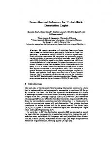
[47, 36]. RV models treat the parameters of a fracture mechanics model as random variables, and assume deterministic crack growth given a realization of these parameters. For this reason, RV models are sometimes also referred to as random growth law models. RP models, also called evolutionary models, assume that each individual crack history is a sample path of a time, cycle count, or spatially indexed stochastic process. 2.2.2.1 Random Variable Models A RV model is formulated by identifying parameters that contribute significantly to the variability in fatigue life and recasting them as a jointly distributed random vector. A parameter’s contribution to the overall variability of fatigue life is assessed with a sensitivity analysis and determination of the magnitude of the uncertainty in its value. A crack is assumed to grow deterministically according to a single realization of the random crack growth parameter vector. Under these assumptions, the distribution of the cycles to a given crack length is determined by propagating the parameter uncertainty through the deterministic model. The first random variable models assumed that the uncertainty in the cycles to crack initiation dominates the uncertainty. For HCF applications, this assumption may be reasonable since the majority of the fatigue life is occupied by crack initiation. Johnson et al. investigated the distribution of crack initiation times for panels on a military transport aircraft [35]. The distribution of crack initiation times is of little practical use since the initiation life depends strongly on the applied load spectrum as noted by Yang [82]. Furthermore, the variance in crack initiation times is sensitive to the applied load spectrum. The scatter in initiation times is especially large for components experiencing low stress amplitudes with few initial defects. Sinclair and Dolan demonstrated the increased scatter in fatigue life at low stress levels in a series of tests on identical highly-polished 7075-T6 aluminum specimens cycled at
17
six different stress amplitudes [63]. Sobczyk and Spencer explain this observation by noting that initiation of cracks from defects at low stress levels may be more sensitive to the random microstructure, leading to increased variability [64]. Yang describes a more useful quantity, the equivalent initial flaw size (EIFS) distribution, defined as the distribution of crack sizes at some reference time. The EIFS distribution allows arbitrary load sequences to be considered in the analysis. Fawaz performed numerous tests investigating the EIFS distribution for aluminum lap joints [20, 21], and DeBartolo and Hillberry performed a microscopy study of the distribution of flaw sizes and shapes in aluminum alloys [14]. Other probabilistic fatigue studies have assumed a random EIFS, such as White et al. [75], Maymon [48], and Luo and Bowen [42]. The data set by Virkler et al. [69], shown in Figure 3, demonstrates that simply randomizing the initial conditions, either through initiation times or EIFS, is insufficient to capture the full variability in fatigue crack growth. Significant variability in crack growth histories was found in tests on 68 identical specimens starting from the same initial crack length. Observations such as these motivated a random growth law approach to capture this uncertainty. This is often done by randomizing selected variables that define the relationship between the crack growth rate and stress intensity range. Common random growth laws are based on randomization of constants in the Paris equation, piecewise-linear models, and the SINH crack growth model [38]. 2.2.2.2 Random Process Models While conceptually simple, RV models models fail to capture the variability within an individual crack history because of the deterministic growth assumption. If the within-specimen variability is significant, random process (RP) modeling becomes a more appropriate choice. RP models assume each crack history is a single realization of a time, cycle count, or crack length indexed stochastic process. This is commonly
18
50 Virkler Data Set
Crack Length (mm)
45 Center Crack Specimens 40 2024−T3 Al 35 558.8 mm long 152.4 mm wide 30 2.54 mm thick 25 R = 0.2 Max Load = 23 kN 20 15 10 5 0
0.5
1
1.5
2
2.5
3
Cycles
3.5 5
x 10
Figure 3: Virkler data set [69]
Virkler Crack Velocity Data −2
da/dN (mm)
10
Center Crack Specimens −2024−T3 Al 558.8 mm long 152.4 mm wide 2.54 mm thick
−3
10
Max Load = 23 kN R = 0.2
−4
10
2.5
2.7
10
10
∆K (MPa mm1/2) Figure 4: Virkler crack velocity data [69]
19
2.9
10
done by multiplying the deterministic crack growth rate by a suitable stochastic cycle count or crack length indexed process, denoted X (N ) and Y (a) respectively, as in Lin and Yang [40] and Ortiz [54, 55]. The crack length or cycle time process is then found by integration. For example, a crack length indexed RP model can be written as in Equations 7 and 8.
1 f (∆K (a) , θ) Y (a) Z a Y (a) da N (a) = a0 f (∆K (a) , θ) da dN
=
(7) (8)
Cycle count or time indexed random processes are often simpler to implement because the choice of index leads to a differential equation that allows separation of the deterministic growth function from the random process as in Equations 9 and 10. Yang and Manning have developed a RP model based on a covariant stationary lognormal process with unit median multiplying the deterministic growth rate [83]. Their model’s capabilities for fitting data were further demonstrated by Wu and Ni [79, 80] and Cross et al. [11].
Z
da dN a(N ) a0
da f (∆K (a) , θ)
= X (N ) f (∆K (a) , θ) Z N = X (N ) dN
(9) (10)
0
Crack length or spatial indexed random processes are more difficult to implement than time or cycle count indexed processes. However, they do possess some significant philosophical and practical advantages. Kozin demonstrated that treating crack length as the independent variable leads to a more consistant probabilistic reformulation of the Paris equation [36]. Ortiz noted that under a known loading history the dominant source of crack growth variability is inhomogeneity within the material [54]. Thus, the assumption of a spatial or crack length indexed random process model is 20
a more physically relevant and generalizable approach to evolutionary fatigue crack growth modeling. Ortiz [54, 55], Dolinski [15, 16], and Cross et al. [11] have derived and applied crack length indexed random process models to experimental data.
2.3
Inference of Probabilistic Failure Models
A key step in creating an accurate model is the proper inference of parameters from the results of experiments. The inference methods for different model classes can take notably different forms. RV models require inference of the joint distribution of the model parameters. RP models require that the spectral properties of the crack growth process be characterized. Established statistical methods are employed to perform these tasks when possible. However, several special techniques have been developed in the course of stochastic fatigue modeling research. 2.3.1
Random Variable Model Inference
For random growth law models, a sample set of the random growth law parameters can be obtained by performing a series of regressions in the log da/dN − log ∆K space, one per crack in the data set. For example, if a randomized Paris equation formulation is used, samples of the constant multiple and exponent are obtained by performing a sequence of linear regressions on the crack velocity data in the log da/dN − log ∆K space [81]. This approach may be expanded by performing a series of generalized linear model (GLM) regressions assuming a crack growth law model of the form µ
da log dN
¶ = i
X
βj hj (∆Ki , Ri , ∆Kth , Kc , ...) + σ²i
(11)
j
where hj (·) is some function of relevant crack growth parameters and ²i is a zeromean Gaussian error term. Cross et al. analyzed the Virkler data using a polynomial GLM [11]. Non-linear regressions can be performed for piecewise-linear growth laws as in
21
Bigerelle et al. [6] and Righiniotis and Chryssanthopoulos [59]. Similarly, regressions for curvilinear growth laws, such as the SINH law, can be performed as in Cross et al. [11] and Yang et al. [84]. A multivariate distribution can then be fit to the growth law parameter samples. Predictions can be made by propagating the parameter uncertainty through the crack growth model. To solve for a random EIFS or crack initiation time from an individual crack history, the appropriate crack growth model is used to grow the crack backwards to a reference time. However, doing so requires that the crack growth rate parameters be known with certainty, which is seldom the case. Makeev et al. noted that if the variability of the crack growth rate is not accounted for, the inferred EIFS distribution will contain variability due to growth rate and hence be overly conservative [45]. Furthermore, the EIFS distribution will not be generalizable to other experimental conditions since it was inferred from a specific combination of uncertainties. Makeev et al. provide a method to infer a data set independent EIFS distribution when a known uncertaintly is present in the crack growth rate. Cross et al. used Bayesian techniques to extend Makeev’s method to perform simultaneous EIFS and growth law inference when the variability in the crack growth rate is unknown [12]. 2.3.2
Random Process Model Inference
Inference of RP model parameters is inherently more complicated than RV model inference because the properties of a stochastic process must be determined. Usually the mean or median behavior of the stochastic crack history process is assumed to be that predicted by fracture mechanics analysis. The autocovariance function, or equivalently the power spectral density (PSD), however, must be determined from analysis of real crack growth histories. For situations where the data are evenly spaced in the index set of the random process, this can accomplished by determining an average spectrum of time or crack length series data and fitting a curve to obtain a
22
functional form for the PSD as done by Ortiz [54, 55]. The stationary autocovariance function is found by taking the inverse Fourier transform of the PSD. Alternatively, a parametric functional form for the autocovariance function can be assumed based on experience or preliminary analyses. Using the expression for the autocovariance, the mean and variance of the life to a given crack size can be calculated. Yang and Manning approximated the distribution of component life from a time indexed stochastic process using a lognormal distribution with the mean and variance calculated using the autocovariance function [83]. Cross et al. found that point estimates for the autocovariance parameters can be inferred by assuming independence of each observation and performing a maximum likelihood estimation (MLE) using the lognormal approximation [11]. They then calculated confidence intervals for the parameters using a block bootstrap method to properly capture the statistical dependence between observations.
2.4
Bayesian Inference and Updating of Failure Models
The distributions of probabilistic fatigue model parameters are seldom known a priori and must be inferred from material and structural tests. In addition, the results of further experiments after the first model inference provide information that should be used to update knowledge of these distributions. An intuitive way to model these uncertainties explicitly is with a probability distribution function. Prior probability distributions modeling the uncertainty of model parameters can be systematically updated using Bayes’ theorem [27]. Bayes’ theorem, shown in Equation 12, gives an expression for the posterior probability distribution of a random event, A, given data, D, in terms of a prior distribution, π (A) for the event of interest and the likelihood of the data given that A occurs, L (D|A). The posterior distribution constitutes an updated statement of the degree of belief in the true values of the underlying random quantities.
23
L (D|A) π (A) L (D|A) π (A) dA A
P (A|D) = R
(12)
Since the data in a Bayesian updating problem is given, D represents a realization of the data and not a random quantity. Therefore the marginal probability of D is a constant implying that the numerator in Equation 12 is constant as well. For this reason, the denominator may be ignored and Equation 12 may be rewritten as
P (A|D) ∝ L (D|A) π (A)
(13)
In Bayesian updating, the current estimate of the fatigue crack growth model parameters’ distribution should be used for the prior distribution. If no suitable prior information exists, a non-informative or vague prior distribution may be assumed [12]. Care must be used if an improper non-informative prior distribution is specified to ensure that the posterior distribution is proper [27]. The likelihood distribution can be derived from the particular probabilistic fatigue model. In addition to inferring the probabilistic growth model, the distribution for life of a single structural component can be updated based on its own repair and inspection history. This allows maintenance and inspections to be individually tailored to each component based on its own condition. Zhao and Haldar developed a Bayesian updating method that accounts for inspection and repair results based upon a Gaussian approximation of the distribution of reliability indices [86]. However, it must be noted that their method implicitly assumes that all necessary parameters and distributions used to predict the reliability index are known. Thus they assume the results of inspections contribute negligibly to the knowledge of the reliability distribution. A similar assumption was made by Madsen in updating reliability estimates with inspection data to quantify the failure probability given survival to a specified usage [43]. Assuming the true life distribution is known with certainty, Equation 12 gives 24
the updated reliability simply as the prior probability of survival to the extended lifetime divided by the probability of surviving the observed usage. The assumption of certainty in the distribution of component life in many applications cannot be supported. Schedule and cost constraints often preclude the extensive testing required to make the uncertainty in the fatigue life distribution negligible. For example, the S-N curve and coefficient of variation in fatigue life for rotorcraft dynamic components may be determined by experiments on as few as five specimens in practice. Because of this, maintenance data also provides information on the fleet-wide component life distribution, reducing epistemic uncertainty. Cross et al. demonstrated reduction of conservatism in fatigue life predictions due to updating of fleet-level parameters [10].
25
CHAPTER III
BAYESIAN FORMULATION 3.1
Hierarchical Bayesian Updating Formulation
Proper construction of the Bayesian reliability model requires that a distinction between component-level information and fleet-level information be made. Componentlevel information pertains to individual realizations of random parameters and processes for a specific component. Fleet-level information describes the uncertain probability distributions for these parameters and stochastic processes. The natural hierarchy created by the distinction between component-level and fleet-level information fits well into the Bayesian framework. A natural way to select probability laws for component-level random quantities is through distributions conditional on the values of fleet-level variables. In this manner, the fleet-level variables behave as hyperparameters that specify the probability distributions of the component-level variables. Let Di and Θi denote the set of all observations and set of random componentlevel parameters for the ith of Nc components, respectively. Assuming statistical independence between observations of distinct components, the likelihood function of the set of all data gathered can be expressed as
L (D = {Di : i = 1 . . . Nc } |θi : i = 1 . . . Nc ) =
Nc Y
Li (Di |θi )
(14)
i=1
Note that statistical independence of observations of the same component is not necessarily assumed. Also note that each component may have its own likelihood function for its data set, as indicated by the subscripted notation, Li . The hierarchy of information also allows the prior distribution of Θi to be expressed conditionally as πΘ|A (θi |α). Since statistical independence may be assumed between 26
components, the prior distribution for all component-level random variables can be expressed as a product similar to that in Equation 14. The final distribution to be specified is a hyperprior distribution for A, denoted πA (α). This distribution models the a priori epistemic uncertainty in the probabilistic law for the component-level parameters. Using Bayes’ rule, the likelihood, prior, and hyperprior distributions are used to compute the posterior distribution of the fleetlevel and component-level parameters, given all data as
πA,Θ|D (α, θi : i = 1 . . . Nc |D) ∝ πA (α)
Nc Y
Li (Di |θi ) πΘ|A (θi |α)
(15)
i=1
Equation 15 represents the joint distribution of all parameters conditional on the observed component data. Several useful distributions may be calculated from the full posterior distribution. First, marginal distributions for the hyperparameters and individual parameter sets are found by integration as
Z
Z
πA|D (α|D) =
··· θ1
Z Z πΘk |D (θk |D) =
πA,Θ|D (α, θi : i = 1 . . . Nc |D) θNc
Nc Y
(16)
i=1
πA,Θ|D (α, θi : i = 1 . . . Nc |D) dα α
dθi
θi ,i6=k
Y
dθi
(17)
i6=k
Next, several posterior predictive distributions of interest can be calculated from the marginal distributions in Equations 16 and 17. The distributions of some function g (Θ) for an inspected and uninspected component are given in Equations 18 and 19, respectively, where δ (·) denotes the Dirac delta function. Setting g (Θ) = Θ in Equations 18 or 19 gives the posterior predictive distribution for the inspected and uninspected component level parameters, respectively. Specifying g (Θ) in Equation 18 to be the remaining life of a component gives the posterior residual life distribution for each inspected component.
27
Z πg(Θi )|D (g|D) =
δ (g − g (θi )) πΘi |D (θi |D) dθi Z Z πg(Θ)|D (g|D) = δ (g − g (θ)) πΘ|A (θ|α) πA|D (α|D) dαdθ
(18)
θi
θ
(19)
α
Thus far the likelihood and prior distributions have been only referenced in general terms. The following discussions describe specific details for the specification of likelihood and prior distributions. 3.1.1
Likelihood Function Determination
Observations of components can be separated into categories, crack detection and crack measurement, that determine the form of the likelihood function. It is assumed in this work that the error characteristics of the inspection methods and measurement techniques are known. For a crack growth model formulation, it is also assumed that the form of a crack growth model, N (a, θ), and its inverse, a (N, θ), are provided where a represents the final crack length, and N the number of cycles. The requirements on the crack growth model are general, only requiring that it can be inverted and that it is completely specified given a realization of the random parameters, θ. Similarly, when a safe-life model is used, it is assumed that a crack growth model, t (θ), is given. When a crack growth model is used, the error in a crack detection inspection is characterized by a probability of detection (POD) curve that gives the likelihood of detecting a crack of length a present in the specimen. A data set obtained from a set of Nc components, each inspected once, can expressed as D = {Di = (Ni , di ) : i = 1 . . . Nc } where di is an indicator variable that equals unity if a crack was detected and zero otherwise. The likelihood of an element Di can be expressed as
Li (Di |θi ) = 1 − di + (2di − 1) POD(a (Ni , θi ))
28
(20)
When a safe-life formulation is used, the data set can be expressed as D = {Di = (ti,1 , ti,2 ) : i = 1 . . . Nc } where ti,1 denotes the time of the last inspection with no crack detected, and ti,2 denotes the first inspection time at which a crack is detected. If a crack is detected on the first inspection, ti,1 is set to zero. Likewise, if no crack is ever detected, ti,2 is set to infinity. The likelihood function of a data point can thus be expressed as
L (Di |θi ) = 1 [ti,1 ≤ t (θi ) ≤ ti,2 ]
(21)
where 1 [·] is the indicator function that equals one if its argument is true and zero otherwise. For a crack measurement inspection, it is assumed that the distribution of measurement error can be written conditionally on the true crack length as fE (e|a). A data set gathered from from Nc components, each inspected once, is expressed as D = {Di = (Ni , ai ) : i = 1 . . . Nc } where ai denoted the measured crack length. The likelihood function of a datum is written as
Li (Di |θi ) = fE (ai − a (Ni , θi ) |a (Ni , θi ))
(22)
The likelihood of the entire data set is then calculated using Equation 14. Generalization of Equations 20 and 22 to cases where components are inspected multiple times is straightforward. 3.1.2
Prior Distribution Specification
Standard parametric distributions provide a flexible means to model the uncertain distribution of fatigue model parameters. Use of parametric forms allows the uncertainty in the distribution itself to be represented by the distribution of hyperparameters that specify the prior distribution. Two-parameter distributions such as the Weibull, normal, and lognormal have hyperparameters that permit uncertainty in both location 29
and scale. Selection of distribution will depend on the specific random quantities to be modeled. Details to consider include skewness, domain, and practical computational concerns. For example, the normal distribution should not be used to model an EIFS distribution since negative EIFS values have no physical meaning. Similarly, a lognormal distribution should not be used to model a left-skewed random variable. Computational considerations may enter into the prior selection when the likelihood function admits a conjugate or semi-conjugate prior. Applying Bayes’ rule to a conjugate likelihood prior pair results in a posterior distribution of the same form as the prior. Semi-conjugate pairs combine under Bayes’ rule to yield a posterior distribution in which the full conditional distributions have the same form as the individual variates’ priors. Obtaining the full conditionals can simplify posterior sampling simulation. It must be noted that the complexity of the likelihood functions previously described seldom admits conjugate priors. 3.1.3
Hyperprior Distribution Specification
The uncertainty in the fatigue model parameter distributions themselves is captured by regarding the hyperparameters that specify these distribution as uncertain. The hyperprior distribution should reflect all prior information, or lack thereof, on the hyperparameters. Prior information may come from previous experiments or possibly expert opinion. Except in special cases, a proper, i.e. integrable, distribution should be used to ensure that full posterior distribution is proper as well. No meaning can be assigned to an improper posterior distribution since it cannot be normalized and integrated to make probability statements. Thus true non-informative priors may not be appropriate in this study unless integrability can be proven. Lack of prior information may be modeled by diffuse hyperpriors that approximate a non-informative prior over the feasible region of values.
30
When previous information or belief is not available on the hyperparameters, an empirical Bayesian approach may be adopted to elicit hyperprior distributions. Point estimators of hyperparameters can be determined by using approximate techniques such as pooled data regression or one-factor-at-a-time inference techniques. The particular estimation technique depends on the hyperparameters to be determined. Hyperprior distributions may be set with mean value equal to the point estimate and standard deviation equal to the standard error, if available.
3.2
Posterior Simulation Schemes
Within the Bayesian philosophy, the posterior distribution represents a model of the uncertainty in the random quantities of interest given available data and prior belief. Hence, point estimation as in frequentist methods is not consistent with the Bayesian statistical paradigm, which treats the parameters as random variables rather than unknown constants. Characterization of the posterior distribution is required to obtain credible intervals for the values of parameters of interest. In this application, the hierarchical structure of these models generally leads to complex joint distributions with numerous parameters of interest, preventing analytical posterior analysis or direct sampling in most cases. This section presents several posterior characterization schemes that are employed in this research. 3.2.1
Rejection Sampling
Among the simplest algorithms for sampling an arbitrary distribution is the rejection sampling technique [27]. Let p (θ|y) denote the (possibly un-normalized) posterior density function, and let g (θ) denote a (possibly un-normalized) distribution function that can be directly sampled. If a distribution g (θ) can be identified such that there exists some finite M such that
sup θ
p (θ|y) =M j , D
(35) (36)
An iteration of a Gibbs sampling simulation begins by generating a sample of the first of the parameters, θ1 , from Equation 35, given the most recent samples of the remaining random parameters. The iteration continues sampling sequentially the remaining random quantities in the random vector, conditioned on the most recent samples, using Equation 36. Posterior distributions that admit practical Gibbs samplers may be formulated using conditionally conjugate distributions for the likelihood and priors. Use of conditionally conjugate distributions results in a posterior distribution for which the full conditional distributions take a standard form. Gelman et al. provides numerous examples of conjugate and semi-conjugate likelihood and prior distribution pairs [27]. An important conjugate pair for analyzing generalized linear models (GLM) in this research consists of multivariate normal likelihood with a batch diagonal covariance matrix, multivariate normal prior for the mean vector, and inverse gamma density for the variance priors. The batch diagonal covariance matrix can be written as
Σ=
σ12 In1
σ22 In2 ..
.
(37)
σp2 Inp where nk , p, and In denote the number of observations in block k, the number of blocks, and the identity matrix of size n, respectively. The GLM for the vector of observations, Y, may be expressed in matrix form as 36
Y|β, σi2 : i = 1 . . . p ∼ MVN (Xβ, Σ)
(38)
where X denotes the matrix of explanatory variables and β denotes the vector of unknown regression coefficients. The conditionally conjugate priors are normal and inverse gamma given as
β ∼ MVN (µβ , Σβ ) σi2 ∼ IG (νi , γi )
(39) (40)
where Σβ is a batch diagonal covariance matrix of size m × m. Note in this work that the inverse gamma density is parameterized as
³ γ´ γν X ∼ IG (ν, γ) ⇔ fX (x) = exp − Γ (ν) xν+1 x
(41)
Following Gelman et al. [27], the prior information can be regarded as additional data, allowing Equations 38 and 39 to be combined as
Y0 |β, σi2 : i = 1 . . . p ∼ MVN (X0 β, Σ0 )
(42)
where
Y Y0 = µβ X X0 = Im Σ 0 Σ0 = 0 Σβ 37
(43)
(44)
(45)
A standard exercise gives the full conditional equations as
³ ´ ˆ V β|σi2 : i = 1 . . . p, Y ∼ MVN β, µ ¶ ni s2i 2 σi |β, Y ∼ IG νi + , γi + 2 2
(46) (47)
where
βˆ = V = s2i =
¡ ¡ ¡
X0T Σ0−1 X0 X0T Σ0−1 X0
¢−1
X0T Σ0−1 Y0
(48)
¢−1
Y0(i) − X0(i) β
¢T ¡
(49) Y0(i) − X0(i) β
¢
(50)
and superscript (i) in Equation 50 denotes the rows of Y0 and X0 corresponding to the ith batch. Although the Gibbs sampler accepts a new sample each iteration, it may be inefficient at traversing the entire probable domain of the posterior distribution in cases of strong posterior statistical dependence between random variates. To see this, consider a bivariate normal distribution with correlation coefficient near unity. Given one variate, only a small fraction of the marginal domain of the other has significant conditional probability mass. Hence, the sampler will only take small steps relative to the size of the likely domain of each variate. Random variable transformations may be employed in some applications to overcome this difficulty. Note that since the Gibbs sampler is a MCMC algorithm, a stationary state of simulation must be achieved before samples can be considered to be drawn from the posterior distribution. Hence the simulation must be burned in and a convergence assessment must be performed. For Gibbs sampler simulations, the posterior samples must be analyzed for statistical dependence between variates and serial correlations between successive samples. Strong autocorrelations or cross-correlations between 38
variates may indicate a poor simulation since statistical dependence effectively reduces the sample size.
3.3
Simplified Hyperparameter Updating
Implementation of probabilistic model updating for practical applications motivates development of simplified techniques to avoid the requirement for an expert user to perform the analysis. Posterior mode approximations using the multivariate normal distribution enable closed-form approximate updating techniques. First, a multivariate normal approximation is fit to the posterior distribution of the appropriately transformed hyperparameter vector. Let T (A) denote the transformation and π ˜T(A)|D (T (α) |D) denote the multivariate normal approximate distribution of the transformed hyperparameters. An effective technique to create the initial approximation is first to transform the hyperparameter samples from a simulation, then to calculate the mean vector and covariance matrix of the transformed samples. Next, assume an additional data, denoted D0 , is received for M additional uninspected components. Let Θ0i denote the component-level parameter vector ith of these M components. Using Bayes’ rule, the updated distribution, given both D and D0 , for the transformed hyperparameters can be expressed as
π ˜
T(A)|D,D 0
0
(T (α) |D, D ) = π ˜T(A)|D (T (α) |D)
M Y
Li (Di0 |α)
(51)
i=1
where the evidence of the hyperparameters is computed for each datum by integration as Z Li (Di0 |α)
= θi0
Li (Di0 |θi0 ) πΘ|A (θi0 |α) dθi0
(52)
In a manner analogous to maximum likelihood estimation, the logarithm of the posterior distribution in Equation 51 is then maximized over all feasible values of the 39
transformed hyperparameter vector using a gradient-based method. The updated mean can then be approximated as à E [A|D, D0 ] ≈ arg max log π ˜T(A)|D (T (α) |D) + T(α)
M X
! log Li (Di0 |α)
(53)
i=1
and the updated covariance matrix can be estimated as the negative inverse of the Hessian matrix of the log-posterior evaluated at the maximum. The remaining component is efficient estimation of the evidence integrals in Equation 52. When the dimension of Θ0 is small enough, discretization-based integration techniques may be employed over a finite feasible region of Θ0 to compute a numerical estimate of the evidence. For higher dimensional integrals, accelerated sampling techniques, such as Latin hypercube or weighted-importance sampling, may be used to estimate the evidence efficiently.
40
CHAPTER IV
UPDATING OF HIGH-CYCLE SAFE-LIFE MODELS 4.1
Description of Input Data
The following considers the updating of a probabilistic initiation life model under HCF spectrum loading for a notional helicopter dynamic component with maintenance findings. The notional data for this section was made available through research conducted by The Boeing Company and Sikorsky Aircraft Corporation [44]. The highcycle load spectrum experienced by the notional component per hour of operation is presented in normalized form in Table 1. The notional maintenance data consist of an inspection time, the results of a crack detection inspection, and corrosion pit depth measurement, if corrosion is present. The maintenance findings for components subjected to Smax = 124.1 MPa are presented in Table 2. A probabilistic stress-life model [44] is provided for the cycles to failure, N , of the components under constant stress amplitude, Sa , loading as
Sa β = 1+ γ C (d) E∞ N
(54)
where β, γ, and the endurance limit, E∞ , are assumed to be jointly distributed random variables defining the S-N curve, realized once per component. The function C (d) in Equation 54 represents an empirical knockdown factor on the endurance limit, E∞ , as a function of a random corrosion pit depth measured in millimeters, d, initiating at a random initiation time, T . The form of this knockdown factor is given in Equation 55.
41
Table 1: Normalized high-cycle spectrum for helicopter dynamic component Sa /Smax 1.000 0.880 0.760 0.723 0.720 0.680 0.668 0.640 0.600 0.560 0.520 0.481 0.480 0.472 0.448 0.440 0.400 0.388 0.381 0.367 0.360 0.347 0.324 0.320 0.293 0.280 0.261 0.247 0.240 0.200 0.160 0.120 0.080
Cycles Per Hour 1 1 1 6 2 8 1 20 231 1419 4230 3034 134 68 108 716 272 67 74 67 155 67 34 142 67 154 68 67 95 59 14 66 215
42
Table 2: Maintenance data crack and corrosion findings Component Number Time in Service (hrs) 1 750 2 750 3 790 4 800 5 850 6 860 7 875 8 895 9 900 10 920 11 925 12 950 13 975 14 975 15 1000 16 1000 17 1000 18 1020 19 1050 20 1075 21 1100 22 1100 23 1120 24 1120 25 1150 26 1180 27 1200 28 1200 29 1250 30 1300
43
Corrosion Depth (mm) 0 0 0 0 0 0.8128 0 0 0 0 0 0 0 0.2032 0 0 0.8890 0 0.1270 0.7112 0 0 0 0 0 0 0 0.5842 1.0160 0
Crack Detected No No No No No No No No No No No No No No No No No No No No No No No No No No No No Yes No
C (d) =
1.03672 ¡ ¢ 1 + exp d−0.9652 0.2921
(55)
Based on fleet corrosion grind-out data, a Weibull distribution with a shape factor of 1.31 and scale factor of 0.3584 mm is determined for the corrosion depth of a corroded part. Fleet corrosion rate data was analyzed to obtain a Weibull model for corrosion onset times with shape parameter 1.07 and a scale parameter 7.014·104 hours.
4.2
Bayesian Model Construction
Because of the stress-life formulation, a crack detection likelihood function similar in form to Equation 21 is appropriate. Since the total likelihood function is the product of indicator functions, it can only take the values one or zero. The total likelihood thus equals one if the parameter vector for each component gives a life prediction in agreement with that component’s maintenance record and equals zero otherwise. The life prediction function is calculated using the S-N curve in Equation 54 and Miner’s rule, given a realization of the parameter vector. For the ith component prior to corrosion initiation, the damage accumulated per hour is computed as a sum of damage accumulated at stress amplitudes, Sa,j weighted by hourly cycle counts, Nj , obtained from Table 1.
X
∆i (θi ) =
j
½ µ ¶¾γi−1 S a,j Nj βi−1 max 0, −1 E∞,i
(56)
Similarly, after corrosion, the damage per hour accumulated in the ith component is computed as
∆di (θi ) =
X
½ Nj
µ −1 βi max 0,
j
44
¶¾γi−1 Sa,j −1 C (di ) E∞,i
(57)
Combining these results, the life for the ith component can be computed from the parameter vector as
t (θi ) =
∆i (θi )−1
: Ti ∆i (θi ) ≥ 1
£ ¤ Ti + [1 − Ti ∆i (θi )] ∆di (θi ) −1
: Ti ∆i (θi ) < 1
(58)
The logarithmic transformation allows use of the multivariate normal distribution to model the joint prior distribution of the S-N parameters conditional on an uncertain mean vector, M, and covariance matrix, S.
log β γ log E∞
¯ ¯ ¯M, S ∼ MVN (M, S) ¯
(59)
Data driven hyperprior distributions were specified with expected values equal to point estimates of M and S. A multivariate normal hyperprior is assumed for M as
−1.2111 M ∼ MVN 0.7500 , V I3 4.7002
(60)
where I3 is the 3×3 identity matrix and V denotes a variance parameter set according to the prior confidence in the point estimate of M. Higher values of V correspond to high prior uncertainty in the median vector. The Wishart density [77] with n degrees of freedom, given in Equation 61, is assumed for the covariance matrix with expected value equal to the point estimate. Use of the Wishart density ensures that the covariance matrix is positive-definite with probability one as its support consists of all symmetric positive-definite matrices of size p × p.
45
S ∼ W (Σ, n) ⇔ fS (S) ∝ |S|
n−p−1 2
µ
¢ 1 ¡ exp − tr Σ−1 S 2
¶ (61)
The hyperprior for the covariance matrix can be expressed as given in Equation 62. The degrees of freedom are set according to the prior confidence in the point estimate, with higher values of n corresponding to higher confidence.
0.0143 −0.0072 0.0057 nS ∼ W −0.0072 0.0056 −0.0042 , n 0.0057 −0.0042 0.0064
4.3
(62)
Posterior Simulation
Due to the crack detection formulation of the likelihood function and hierarchical model structure, a rejection sampling technique to simulate the posterior distribution was implemented. First, candidate samples of M and S are generated from the hyperprior distributions in Equations, 60 and 62. Next, candidate samples of the S-N parameters, one set per inspected component, are generated from Equation 59 given the candidate samples of M and S. For components on which corrosion was found, a corrosion initiation time, Ti , was sampled from the initiation time distribution, conditional on Ti ≤ ti,insp as
fT (τ ) fTi (τ |Ti ≤ ti,insp ) = R ti,insp i ; τ ∈ [0, ti,insp ] f (s) ds T i 0
(63)
The samples of crack initiation parameters are then used in Equation 58 to calculate candidate samples of the total life for each inspected component, t (θi ). The candidate samples of the hyperparameters and component crack initiation parameters are accepted if the computed lifetimes are in agreement with the inspection results.
46
A rejection sampling simulation of the posterior distribution consisting of 2·105 samples was performed. The variance parameter, V , in Equation 60 is set to 0.01 corresponding to a coefficient of variation (COV) in the prior median (untransformed) values of β, γ, and E∞ of roughly 10%. The number of degrees of freedom in Equation 62 was set to n = 10 resulting in a prior coefficient of variation in the variance of S-N curve parameters of approximately 45%.
4.4
Simulation Results
The rejection sampling simulation yielded 2 · 105 posterior distribution samples for each of the hyperparameters, M and S, S-N parameters for each inspected part, and corrosion initiation time for each corroded part. The marginal posterior distributions for M and S estimated from the samples were compared to their prior distributions in Equations 60 and 62. The prior hyperparameter statistics are compared to their updated values in Table 3. The most significant difference between the prior and updated statistics is the reduction of 23% in the coefficient of variation of E [log E∞ ], the third component in M. The expected updated values of components of M differ from their corresponding prior values by less than 1%. Therefore, the key result of this updating with regard to hyperparameters is the removal of epistemic uncertainty in the median value of the endurance limit, E∞ . Figures 5 and 6 depict this result graphically with a comparison of the prior and updated marginal density functions and distribution functions, respectively. Next, the samples of S-N parameters, corrosion onset times, and corrosion pit depths for inspected components were post-processed to make updated probabilistic life statements about the remaining life of these parts. For each component on which no corrosion was observed, a corrosion depth was sampled from the pit depth Weibull distribution, and an onset time was sampled from the corrosion initiation Weibull distribution, conditional on T > ti,insp .
47
Table 3: Probabilities of crack initiation for at-risk components Prior Value
Updated Value
−1.2111 E [M] = 0.7500 4.7002
−1.2112 E [M|D] = 0.7496 4.7068
0.0825 cov [M] = 0.1333 0.0213
0.0825 cov [M|D] = 0.1333 0.0164
0.0143 −0.0072 0.0057 E [S] = −0.0072 0.0056 −0.0042 0.0057 −0.0042 0.0064
Probability Density
0.06
0.0141 −0.0070 0.0055 E [S|D]= −0.0070 0.0055 −0.0040 0.0055 −0.0040 0.0062
Updated Distribution Prior Distribution
0.05 0.04 0.03 0.02 0.01 0 80
90
100
110
120
130
140
Median Endurance Limit (MPa) Figure 5: Updated and prior density functions for median endurance limit
48
Cumulative Probability
1
0.8
0.6
0.4
0.2 Updated Distribution Prior Distribution 0 80
90
100
110
120
130
140
Median Endurance Limit (MPa) Figure 6: Updated and prior distribution functions for median endurance limit
fTi (τ ) ; τ ∈ (ti,insp , ∞) f (s) ds ti,insp Ti
fTi (τ |Ti > ti,insp ) = R ∞
(64)
With the completed sample set of crack initiation parameters for each inspected component, the distribution of remaining life was calculated for each inspected component, using Equation 58, as t (θi ) − ti,insp . This analysis revealed a set of four components, numbers 6, 17, 20, and 28, whose probabilities of failure within an additional 1,000 service hours are orders of magnitudes higher than the others. These components were termed ”at-risk,” and their computed failure probabilities under continued usage are given in Table 4. This result demonstrates a rational method to assess serviceable damage limits by determining the reliability for continues use of damaged components. In this manner, this reliability analysis can be used as a tool for repair and replacement decisions. Samples of the posterior predictive distribution for the endurance limit were generated from Equation 59 given each sample of the hyperparameters. From these 49
Table 4: Probabilities of crack initiation for at-risk components Component number 6 17 20 28
Probability of Probability of Probability of initiation initiation initiation within 100 hours within 500 hours within 1000 Hours 1.11% 5.26% 8.87% 5.31% 20.3% 29.9% 0.11% 0.62% 1.17% −3 7.5·10 % 0.045% 0.98%
samples, the updated distribution of realized endurance limits for uninspected components was estimated. Figure 7 compares the posterior predictive distribution of the endurance limit to the prior predictive distribution, depicting the narrowing of the distribution due to the consideration of maintenance data. The improvement in precision is also reflected by a 15% narrowing of the 95% credible interval for the endurance limit from [85.5 MPa, 142.0 MPa] to [88.9 MPa, 137.2 MPa]. Note that the posterior predictive distribution for E∞ represents the updated distribution of endurance limits from uninspected components in light of the data obtained for others. Therefore the updating analysis provides relevant information about the uninspected population as well as those components that were inspected. The importance of the narrowing of the predictive distribution becomes apparent when considering the distribution of fatigue lives for uninspected components. By drawing probability mass away from extremely low endurance limits, the updating analysis shows that low component lifetimes are less likely in light of the maintenance data. Since the high-reliability portion of the component life distribution is of central interest, the shift of probability mass in the endurance limit distribution away from the lower tail can have a pronounced effect on the reliability calculation for lifetimes of interest. Figure 8 compares the updated and prior high-reliability portion of the cumulative distribution function for the life of an uninspected component. This rightward shift in substantiated reliability is the result of an updating analysis given thirty
50
Updated Distribution Prior Distribution
Probability Density
0.04
0.03
0.02
0.01
0 80
90
100
110
120
130
140
Endurance Limit (MPa) Figure 7: Posterior and prior predictive density functions for endurance limit, E∞ inspection data points. A more substantial shift may be achieved if the volume of inspection data approaches that available from a fully-populated fleet maintenance database. The smaller magnitude of the change in reliability for uninspected components versus inspected components is expected. Specific information on the componentlevel parameters for each inspected component is obtained from its own maintenance records, whereas only fleet-level information can be applied to predictions of the reliability for uninspected components. Since the component-level parameters govern the fatigue life directly, more significant changes in reliability should occur for inspected components as observed here.
51
Cumulative Probability of Failure
−3
5
x 10
4
Updated Distribution Prior Distribution
3 2 1 0 0
2000
4000 6000 Fatigue Life (hrs)
8000
10000
Figure 8: Updated life distribution for uninspected components
52
CHAPTER V
EQUIVALENT INITIAL FLAW SIZE INFERENCE 5.1
Description of Input Data
Following Cross et al. [12], the growth of a double corner crack from a rivet hole in a 2024-T3 Aluminum fuselage lap joint is considered. Figure 9 illustrates the crack geometry. The skin is 1.016 mm thick with 4.76 mm fasteners spaced every 27.2 mm. The US Air Force fracture mechanics based life prediction program, AFGROW [32], is used to calculate the median crack growth behavior under spectrum loading. Based on finite element results from Fawaz and Harter [22], 0.61 tension, 0.85 bending, and 2.61 bearing stress factors are used as inputs to AFGROW. A simulated data set of 20 initial cracks was generated from a Weibull distribution with a scale factor of 1.016·10−2 mm and a shape factor of three. Likewise, a simulated set of 20 multiplicative crack growth rate noises was generated from a lognormal distribution with log-mean of zero and a log standard deviation of 0.1. From these samples, the simulated data set of 20 cracks depicted in Figure 10 was generated using AFGROW.
5.2
Bayesian Model Construction
The uncertain crack growth parameters for this problem are the initial flaw size, c, and the growth rate noise, X for which a Weibull and a unit-median lognormal prior prior distribution are assumed, respectively. Thus there are three hyperparameters: the Weibull shape α, Weibull scale β, and log-standard deviation σ. Let N (a, c) denote the number of cycles predicted by AFGROW to grow a crack from the initial flaw size, c, to the observed final crack length, a. The collection of all observed
53
4.76 mm
1.016 mm
Initial Crack Radius Figure 9: Double corner crack from lap joint rivet hole
5.5
Crack Size (mm)
5 4.5 4 3.5 3 2.5 2 0
2
4
6
Number of Cycles
8 4
x 10
Figure 10: Simulated lap joint crack inspection data set
54
final crack lengths and cycle counts will be denoted D = {(ai , Ni ) : i = 1 . . . 20}, and Θi = (ci , Xi ) denotes the vector of uncertain crack growth parameters for the ith crack. Assuming negligible inspection error, the likelihood of the collection of data given all component-level parameters can be expressed as
L (D|Θi ; i = 1 . . . 20) =
20 Y ¡ ¢ δ Xi−1 N (ai , ci ) − Ni
(65)
i=1
A proper vague hyperprior is assumed for the hyperparameters A = {α, β, σ} so that their logarithms are approximately uniformly distributed over the feasible region. All hyperparameters are assumed a priori to be mutually statistically independent. The prior distribution for β is assumed to be Weibull with a scale parameter of one and a shape parameter of 0.01. The prior distributions for α and σ are assumed to be lognormal with log-means Mα and Mσ and log-standard deviations of Sα and Sσ . The values of Mα and Mσ are set using the best available knowledge on the locations of α and σ. The parameters Sα and Sσ are set to be as large as possible without allowing significant probability mass at unreasonable values of the hyperparameters. Since no a priori knowledge of α or σ is assumed, a standard EIFS inference is used as an empirical procedure to elicit the hyperprior distribution location parameters. First, the crack growth model is inverted to obtain a set of point estimates of the initial flaw sizes as C = {ci : N (ai , ci ) = Ni , i = 1 . . . 20}. A Weibull distribution is then fit to the elements of C to obtain estimates α ˆ and βˆ of the shape and scale parameters, respectively. Samples of the lognormal noise in the crack growth rate can be obtained assuming the median initial flaw size for all cracks as o n ³ ´ α ˆ −1 −1 ˆ X = Xi = N ai , β (ln ln 2) · Ni . The hyperprior location parameters are then calculated by the method of moments.
55
Mα = ln α ˆ v u 20 u1 X ¡ ¢2 ln Xi − ln X Mσ = ln t 19 i=1
(66) (67)
The values of Mα and Mσ were calculated as 0.385 and -1.88 respectively, and the dispersion parameters Sα and Sσ were both set to 0.8. The full posterior distribution can then be written as
πA,Θ|D (α, β, σ, ci : i = 1 . . . 20|D) ∝ πA (α, β, σ)
20 Y
L (Ni |ai , ci , σ) πC|A (ci |α, β) (68)
i=1
where " µ µ ¶2 ¶2 # exp (−β 0.01 ) 1 ln α − Mα 1 ln σ − Mσ πA (α, β, σ) ∝ exp − − (69) αβ 0.99 σ 2 Sα 2 Sσ ¶ µ ln Ni − ln N (ai , ci ) −1 (70) L (Ni |ai , ci , σ) ∝ σ φ σ · µ ¶α ¸ ci α α−1 πC|A (ci |α, β) = αβ ci exp − (71) β and φ (·) denotes the standard normal density function.
5.3
Posterior Simulation
The posterior distribution was simulated using MCMC with the Metropolis-Hastings algorithm for the state transition rule. Candidate samples are generated according to an independent lognormal random walk process. Let Yi denote the random vector containing the twenty EIFS and three hyperparameter values in the ith sample. The components of the proposal vector Z are generated according to the distribution
¡
¢ i
qj zj |yj
"
1 ∝ zj−1 exp − 2 56
µ
ln zj − ln yji sj
¶2 # (72)
where the sj are free parameters used to tune the sampler. An iteration of the algorithm proceeds by first generating the candidate vector Z from the distribution in Equation 72. The value of the next sample Yi+1 is generated from the probability distribution ) z j j=1 P Yi+1 = Z = min Q23 i , 1 i πA,Θ|D (Y |D) j=1 yj ¡ i+1 ¢ ¡ i+1 ¢ i P Y =Y = 1−P Y =Z ¡
¢
(
πA,Θ|D (Z|D)
Q23
(73) (74)
A simulation consisting of 10 parallel chains of 106 samples each was performed, where the first half of the samples was discarded to eliminate transient effects on the posterior estimates. The convergence metric in Equation 31 was calculated for the hyperparameters as Rα = 1.00754, Rβ = 1.00765, and Rσ = 1.00063.
5.4
Simulation Results
The marginal posterior densities for the EIFS parameters and growth rate standard deviation were estimated from the MCMC samples and appear in Figures 11, 12, and 13. From the figures, the true values of α, β, and σ (3, 1.016 · 10−2 mm, and 0.1, respectively) are seen to lie in areas of high posterior probability mass. Posterior statistics were also computed and are compared to the true values and standard results in Table 5. The posterior mean, median, and mode all provide closer estimates of the Weibull shape parameter, α, and growth rate standard deviation, σ, than the standard EIFS inference predictions. The posterior predictive density for the EIFS can be computed by averaging the Weibull density evaluated for each shape and scale parameter sample. Figure 14 compares the posterior predictive density to the true EIFS density function as well as the density inferred from a standard EIFS analysis. A clear improvement in EIFS distribution is seen in the Bayesian model prediction over the standard EIFS inference. In addition, posterior predictive EIFS statistics are compared to the true statistics 57
Marginal Posterior Density
0.35 0.3 0.25 0.2 0.15 0.1 0.05 0 0
5
α
10
15
Figure 11: Marginal posterior distribution for Weibull shape parameter
Marginal Posterior Density
300 250 200 150 100 50 0 0
0.005
0.01
β (mm)
0.015
0.02
Figure 12: Marginal posterior distribution for Weibull scale parameter
58
Marginal Posterior Density
14 12 10 8 6 4 2 0 0
0.1
0.2
σ
0.3
0.4
Figure 13: Marginal posterior distribution for growth rate standard deviation
Table 5: Comparison of posterior statistics for distribution parameters True Value Standard EIFS Posterior Mean Posterior Median Posterior Mode Posterior Std. Dev. Posterior 95% CI
α 3 1.47 4.07 3.43 2.61 2.37 [1.52, 10.61]
β (mm) σ −2 1.016·10 0.1 −2 1.115·10 0.152 0.958·10−2 0.138 −2 0.940·10 0.137 0.909·10−2 0.132 −2 0.159·10 0.035 −2 −2 [0.699·10 , 1.321·10 ] [0.070, 2.11]
59
140
Bayesian EIFS PDF Standard EIFS PDF True EIFS PDF
Probability Density
120 100 80 60 40 20 0
0.005
0.01
0.015
0.02
0.025
0.03
Initial Flaw Radius (mm) Figure 14: Posterior predictive equivalent initial flaw size distribution Table 6: Equivalent initial flaw size statistics comparison True Value Standard EIFS Posterior Pred.
Mean (mm) 9.07·10−3 10.0·10−3 8.66·10−3
Std. Dev. (mm) 3.30·10−3 6.96·10−3 3.66·10−3
95% CI (mm) [2.97·10−3 , 1.57·10−2 ] [9.14·10−4 , 2.72·10−2 ] [2.54·10−3 , 1.71·10−2 ]
and standard EIFS statistics in Table 6. The posterior predictive mean and standard deviation differ from the true values by 4.5% and 10.9% respectively, and the 95% credible interval width differs from the true width by 14%. For comparison, the standard EIFS method overstates the mean and standard deviation by 10% and 111%, respectively. The 95% interval predicted by the standard EIFS method is 106% wider than the true value. The hyperparameter samples were then used to generate predictive samples of the crack growth parameter vector (c, X). These predictive samples were then propagated through AFRGOW to obtain samples from the distribution of crack growth histories.
60
5
Crack Size (mm)
4.5
4
3.5 Mean Behavior Target Data 95% Credible Set
3
4
5
6
7
8
Number of Cycles
9
10 4
x 10
Figure 15: Posterior predictive distribution for crack growth history The mean growth history and 95% credible interval are compared to the target data in Figure 15. The posterior model fits the data well, with 19 of 20 data points falling within the 95% credible region, as expected.
5.5
Updating Fleet-Level Parameters
Consider now that an additional rivet joint is inspected with a non-destructive inspection with a probability of detection (POD) curve given in Figure 16. The inspection occurs at 104 hours in service and results in a crack detection indication. The approximate updating procedure is conducted using the maximum a posteriori method with multivariate normal approximations for the posterior hyperparameter distribution. Using the logarithmic transformation for α, β, and σ, the posterior distribution determined from the MCMC simulation may be approximated as
61
Probability of Detection
1
0.8
0.6
0.4
0.2
0 0
0.015
0.03
0.045
0.06
0.075
Crack Length (mm) Figure 16: Probability of detection curve
log α ¯ 1.2720 0.2457 −0.0271 0.0574 ¯ log β ¯D ∼ MVN −4.6626 , −0.0271 0.0262 −0.0081 (75) ¯ log σ −2.0133 0.0574 −0.0081 0.0751 Since Θ = (c, X), the integral required to evaluate the likelihood can be computed using a simple two-dimensional integration technique. First, to save computational time the crack growth model was discretized with equal spacing in c and log X and saved in a matrix form as
¡ ¢ aij = a 104 , {ci , Xj }
(76)
The evidence integral is then estimated as
L (D0 |T (A), D) ∝
XX i
j
à µ ¶ µ ¶2 ! α 1 αβ α cα−1 c log X i j i exp − − POD (aij ) (77) σ β 2 σ 62
The function log π ˜T(A)|D (T ({α, β, σ}) |D) + log L (D0 |T ({α, β, σ}) , D) was then maximized, and the Hessian matrix was computed at that point to give the updated hyperparameter distribution in Equation 78.
log α ¯ 1.2070 0.2377 −0.0169 0.0557 ¯ log β ¯D, D0 ∼ MVN −4.5947 , −0.0169 0.0220 −0.0059 (78) ¯ log σ −2.0307 0.0557 −0.0059 0.0752 To verify the approximation, a MCMC simulation was run to provide a comparison for the mean vector and covariance matrix of the hyperparameters. The estimated mean and variance from the MCMC simulation, as shown in Equations 79 and 80 are in close agreement with the MAP rule approximate updating method.
log α ¯ 1.2031 ¯ 0 ¯ E log β ¯D, D = −4.5941 log σ −2.0302 0.0566 log α ¯ 0.2393 −0.0180 ¯ 0 ¯ cov 0.0222 −0.0063 log β ¯D, D = −0.0180 log σ 0.0566 −0.0063 0.0755
5.6
(79)
(80)
Updating Residual Life Distribution
Now consider the situation that the previously described NDI detects no crack after 104 cycles, and denote this observation as D0 . In this situation it is desirable to simultaneously determine the distribution of remaining life as well as update the distribution for α, β, and σ. The likelihood function, given the parameter vector Θ0 = (X 0 , c0 ), can be computed from the POD curve as
¡ ¡ ¢¢ L (D0 |θ0 ) = 1 − POD a 104 , Θ0 63
(81)
The prior distributions are the same as before, with the Weibull prior for c0 and lognormal prior for X 0 . The approximate hyperprior distribution for the transformed hyperparameters in Equation 75 is used to simplify sampling. Because of the form of the likelihood function, rejection sampling can be implemented exploiting the hierarchical structure of the posterior. First, a candidate sample of the hyperparameters is drawn from the hyperprior in Equation 75. Next, candidate samples of the crack growth model parameters are drawn from their respective priors given the candidate hyperparameters. The candidate crack growth parameter samples are propagated through the AFGROW model to determine the likelihood in Equation 81. The candidate sample is accepted with probability equal to the likelihood. After performing the sampling, the updated distribution of remaining life can be calculated by propagating the uncertainty through the crack growth model. The updated distribution of remaining life for a crack to grow to a length of 0.005 inches appears in Figure 17. A rightward shift in the distribution is observed indicating a upward revision in substantiated reliability. This rightward shift is more pronounced at the high reliability region of the life distribution. Figure 18 provides additional detail on the high reliability region. Likewise, the updated distribution for the hyperparameters was approximated from the samples by computing the mean vector and covariance matrix of the transformed hyperparameter samples. These values were then used to derive a multivariate normal approximation to the updated posterior distribution in Equation 82. The decrease in E [log β|D, D0 ] versus E [log β|D] demonstrates that the passed inspection gives evidence that the true EIFS distribution lies slightly to the left of previous predictions.
64
Cumulative Probability
1
0.8
0.6
0.4
0.2 Inspected Component Uninpsected Component 0 0
1
2
3
4
5
Cycles to a = 0.127 mm
6 4
x 10
Figure 17: Updated distribution of remaining life
Cumulative Probability
0.05
0.04
0.03
Inspected Component Uninpsected Component
Increase in substantiated remaining life
0.02
0.01
0 0
2000 4000 6000 8000 Remaining Cycles to a = 0.005 in
10000
Figure 18: Detail on updated distribution of remaining life
65
log α ¯ 1.3008 0.2455 −0.0280 0.0569 ¯ log β ¯D, D0 ∼ MVN −4.6913 , −0.0280 0.0250 −0.0082 (82) ¯ log σ −2.0063 0.0569 −0.0082 0.0747 Extension of these results to multiple inspected components is straightforward due to the assumed independence of components. Additional likelihood terms and component-level prior distributions must be added for each inspected component. The analysis the proceeds in the same manner as demonstrated.
66
CHAPTER VI
HIERARCHICAL GROWTH RATE MODELING 6.1
Description on Input Data
In the following section, a hierarchical probabilistic model of short-crack growth is derived based on data generated by Swain et al. [65]. A series of short cracks were grown under constant amplitude cycling on single edge notch tension (SENT) specimens prepared from 9.5 mm thick AISI 4340 steel plate. Specimens were tested at R levels of -1, 0, and 0.5 with data recorded for 8, 4 and 3 cracks, respectively. The reduced growth rate data appearing in Figure 19 shows a clear dependence of the crack growth rate on the load ratio. Table 7 summarizes the loading conditions, number of growth rate data points, and geometries for each crack.
6.2
Bayesian Model Construction
Because of the effect of the load ratio and the dependence of data observed from the same crack, a hierarchical GLM is hypothesized of the form µ log10
da dN
¶ = log10 Cij + mij log10 ∆Kijk + σi ²ijk
(83)
ijk
where the ²ijk are independent standard normal random variables. This model corresponds to individual Paris-type equations for the j th crack at the ith R level. The vector of logarithms of all growth rate observations, denoted Y thus has multivariate normal density given the vectors of intercepts and slopes, C and m, respectively.
C Y|C, m, σi : i = 1 . . . NR ∼ MVN X , Σ (σi : i = 1 . . . NR ) m
67
(84)
−6
10
−7
da/dN (m/cycle)
10
−8
10
−9
10
−10
R = 0.5 R = 0.0 R = −1
10
−11
10
0
1
10
2
10
10
3
10
1/2
∆K (MPa m ) Figure 19: Crack growth rate data for AISI 4340 steel
Table 7: Data description for AISI 4340 short-crack tests [65] Crack Number
R
1 2 3 4 5 6 7 8 9 10 11 12 13 14 15
0.5 0.5 0.5 0.0 0.0 0.0 0.0 -1.0 -1.0 -1.0 -1.0 -1.0 -1.0 -1.0 -1.0
Smax Geometry (MPa) 585 Corner 585 Surface 585 Surface 385 Surface/Corner 360 Surface 360 Surface 360 Surface 270 Surface/Corner 270 Surface 270 Surface 240 Surface 240 Surface 240 Surface 240 Surface 240 Surface
68
Number of Observations 5 11 11 16 12 2 6 30 13 4 14 3 2 1 7
Semi-conjugate priors are used for the linear model parameters and unknown variances.
log10 Cij |µCi , σCi ∼ N (µCi , σCi )
(85)
mij |µmi , σmi ∼ N (µmi , σmi )
(86)
µCi ∼ N (ηC , τC )
(87)
µmi ∼ N (ηm , τm )
(88)
σi2 ∼ IG (νe , γe )
(89)
2 ∼ IG (νC , γC ) σCi
(90)
2 σmi ∼ IG (νm γm )
(91)
where the set ξ = {ηC , τC , ηm , τm , νe , γe , νC , γC , νm , γm } consists of prior parameters to be elicited. Note that because of a priori independence, it is a simple matter to express the prior for the collection of slopes and intercepts in multivariate normal form in terms of the mean vector Mh = [µC1 , . . . , µCNR , µm1 , . . . , µmNR ]T as
¯ C ¯¯ ¯σCi , σmi : i = 1 . . . NR ∼ MVN (Xp Mh , Σp (σCi , σmi : i = 1 . . . NR )) m
(92)
£ ¤T An augmented vector of regression unknowns β = CT , mT , MT then has the h distribution
Ya |β, σi , σCi , σmi : i = 1 . . . NR ∼ MVN (Xa β, Σa (σi , σCi , σmi : i = 1 . . . NR )) (93) where
69
Ya
Xa
Σa
Y 02N c = ηC 1NR ηm 1NR 0 X = I2Nc −Xp 0 I2NR Σ 0 0 0 0 Σp 0 0 = 0 0 0 τC2 INR 2 0 0 0 τm INR
(94)
(95)
(96)
Without prior data, the hyperprior parameters, ξ may be determined empirically from the data set. Point estimates of µmi and µCi were obtained by performing a series of regressions on pooled data for each stress ratio and are given in Table 8. \ The prior means, ηC and ηm , were set equal to the sample means of the log 10 Cij and m ˆ ij , respectively. Similarly, the standard deviations τC and τm were computed as the sample standard deviations of the point estimates. The mean squared error of the regressions was used as a mean value for the inverse gamma priors for the unknown variances. The complete set of hyperprior parameter values is given in Table 9. Table 8: Point estimates of hyperparameters from pooled-data regressions \ R log m ˆ ij 10 Cij 0.5 -10.4349 2.3363 0.0 -11.5756 2.8992 -1.0 -11.3802 2.4490
70
Table 9: Numerical values for generalized linear model hyperprior parameters Parameter ηC τC ηm τm νe γe νC γC νm γm
Value -11.1302 0.6100 2.5615 0.2978 2.0000 0.5874 2.0000 0.5874 2.0000 0.5874
The posterior distribution is calculated using Bayes’ rule by multiplying the augmented likelihood function in Equation 93 by the variance hyperprior distributions in Equations 89-91. Because of the semi-conjugate formulation, the full conditional distributions can be expressed in closed form for the mean as
³ ´ ˆ V β|σi , σCi , σmi : i = 1 . . . NR ∼ MVN β,
(97)
and variances as Ã
! Nci X X n 1 i σi2 |β ∼ IG νe + , γe + r2 2 2 j=1 k ijk à ! Nci X 1 N ci 2 2 σCi |β ∼ IG νC + , γC + (log10 Cij − µCi ) 2 2 j à ! Nci X 1 N ci 2 , γm + σmi |β ∼ IG νm + (mij − µmi )2 2 2 j where
71
(98) (99) (100)
βˆ =
−1 XT a Σa Xa
¢−1
−1 XT a Σa Ya
¢−1 −1 XT a Σa Xa µ ¶ da = log10 − log10 Cij − mij log10 ∆Kijk dN ijk
V = rijk
¡ ¡
(101) (102) (103)
and Nci and ni denote the number of cracks and data points, respectively, at the ith R level.
6.3
Posterior Simulation
The closed-form full posterior distributions in Equations 97-100 enable Gibbs sampling to characterize the posterior distribution. The simulation was performed by alternately sampling the full mean conditional and full variance conditionals given the latest sample of each. Initial samples of the random parameters and hyperparameters were taken from the corresponding prior and hyperprior distributions. A simulation of 2 · 104 samples was performed, and the first half of the samples was discarded to reduce the influence of the MCMC startup transient. Serial and cross correlations may be used to assess the strength of statistical dependence of successive samples from the Gibbs simulation. Since the mean vector is drawn as a batch, and the full conditional variance distributions are independent, it follows that only the cross-correlations between the mean variates and variance variates need be considered. The maximum absolute cross-correlation between a mean and variance term was found to be 0.4045, verifying that statistical dependence between variates is not large. In addition, the autocorrelation was computed for each random variate being simulated, and the values for each variate are plotted in Figure 20. The autocorrelation plot shows that no significant periodicity arises in the simulation as autocorrelations fall below 0.1 after 4 iterations.
72
1
Auto−correlation
0.8 0.6 0.4 0.2 0 −0.2 0
10
20
30
40
Lag (Number of Samples) Figure 20: Autocorrelations from Gibbs simulation
6.4
Simulation Results
Useful results can be extracted from the samples obtained from the Gibbs simulation by post-processing. Marginal distributions for the hyperparameters are estimated by considering the hyperparameter samples individually. Figures 21 and 22 depict the marginal posterior densities of the mean regression intercepts and slopes, respectively. A clear rightward shift of one unit is observed in the mean intercept distribution for R = 0.5. The differences in the mean slope distributions between different stress ratios are minor. Similarly, the marginal posterior densities for the intercept and slope variances appear in Figures 23 and 24. Little deviation from the prior distributions is observed. This result is expected, however, since the numbers of observed cracks at each stress ratio are small. The largest deviation from the prior distribution occurs for R=-1.0 where the most data was taken. The final marginal hyperparameter posterior distributions are for the regression 73
Marginal Posterior Density
2.5 R=0.5 R=0.0 R=−1.0
2
1.5
1
0.5
0 −12
−11.5
−11
−10.5
µC,i
−10
Figure 21: Marginal posterior densities of mean regression intercepts
Marginal Posterior Density
3 R=0.5 R=0.0 R=−1.0
2.5 2 1.5 1 0.5 0 2
2.5
µm,i
3
3.5
Figure 22: Marginal posterior densities of mean regression slopes
74
Marginal Posterior Density
16 R=0.5 R=0.0 R=−1.0
14 12 10 8 6 4 2 0 0
0.05
0.1
0.15
0.2
0.25
0.3
σ2C,i Figure 23: Marginal posterior densities of regression intercept variances
Marginal Posterior Density
20 R=0.5 R=0.0 R=−1.0
15
10
5
0 0
0.05
0.1
0.15
0.2
0.25
0.3
σ2 m,i Figure 24: Marginal posterior densities of regression slope variances
75
Marginal Posterior Density
35 R=0.5 R=0.0 R=−1.0
30 25 20 15 10 5 0 0
0.05
0.1
0.15
0.2
0.25
0.3
σ2e,i Figure 25: Marginal posterior densities of regression error variances error variances depicted in Figure 25. Clear differences between the distributions at different stress ratios are observed. The average regression error variances at R = 0.0 and R = -1.0 show increases of 320% and 55%, respectively, over the average regression error variance at R = 0.5. Physical meaning can be assigned to this result by interpreting the regression error variance as a quantification of the irregularity in the growth of a single crack. Crack closure processes may explain these differences, since intuitively, crack closure phenomena should introduce randomness into the growth of a single crack. Surface roughness and debris induced closure are the result of the unpredictably irregular pattern of fracture surfaces along the crack face. Plasticityinduced closure also may introduce irregularity since the small crack front intersects a small number of grains, especially for the data points taken at low stress-intensity factors. When few grains are intersected, the growth behavior is more susceptible to the characteristics of the particular grains on the crack front. Posterior means and standard deviations were also computed for the means and
76
Table 10: Posterior AISI 4340 short-crack growth parameter statistics Statistic E p [µC,i |D] var (µC,i |D) pE [µm,i |D] var m,i |D) £ (µ ¤ 2 E σ |D C,i q ¡ ¢ 2 var σC,i |D £ 2 ¤ E σ |D m,i q ¡ ¢ 2 |D var σC,i ¤ £ 2 E σ |D e,i q ¡ ¢ 2 var σC,i |D
R = 0.5 -10.6665 0.2194 2.5163 0.1663 7.6267·10−2
R = 0.0 -11.3562 0.2162 2.6526 0.1898 6.8829·10−2
R = −1.0 -11.4099 0.1784 2.4456 0.1434 8.6906·10−2
7.9903·10−2 6.4350·10−2
6.3325·10−2 6.7742·10−2
6.5715·10−2 6.0300·10−2
5.7437·10−2 4.8996·10−2
6.0320·10−2 1.5653·10−1
4.3324·10−2 7.5912·10−2
1.4625·10−2
3.9649·10−2
1.3996·10−2
variances of the short-crack growth parameters as well as the regression error variances. These statistics are summarized in Table 10. The marginal hyperparameter samples are then used to generate samples of the posterior predictive distributions for the regression slopes and intercepts. For example, the nth sample of mi is generated from a normal distribution with mean and 2 variance equal to the nth samples of µmi and σmi , respectively. The posterior predictive
distributions for the intercepts and slopes appear in Figures 26 and 27, respectively. Here the rightward shift of the predictive intercept distribution for R = 0.5, together with the similarity of the predictive slope distributions, may be given the physical interpretation of a factor of ten increase, on average, in the crack growth rate at R = 0.5. The faster growth rate at R = 0.5 is expected since the tension-tension cycling prevents significant crack closure. Posterior predictive statistics were computed as well from the samples, and these results are summarized in Table 11. The order-of-magnitude increase in the average growth rate at R = 0.5 is supported by the increase in E [log10 Cij |D]. Predictive standard deviations were approximately equal for each stress ratio.
77
Posterior Predictive Density
1.4 R=0.5 R=0.0 R=−1.0
1.2 1 0.8 0.6 0.4 0.2 0 −12.5
−12
−11.5
−11
−10.5
−10
−9.5
log10Cij Figure 26: Posterior predictive densities of regression intercepts
Posterior Predictive Density
1.6 R=0.5 R=0.0 R=−1.0
1.4 1.2 1 0.8 0.6 0.4 0.2 0 1.5
2
2.5
3
3.5
mij Figure 27: Posterior predictive densities of regression slopes
78
Table 11: Posterior predictive AISI 4340 short-crack growth parameter statistics Statistic R = 0.5 E [log C |D] -10.6676 10 ij p var (log10 Cij |D) 0.3550 2.5139 pE [mij |D] var (mij |D) 0.3084
R = 0.0 -11.3529 0.3435 2.6513 0.3194
R = −1.0 -11.4112 0.3389 2.4449 0.2866
Finally, the posterior predictive distribution for the crack growth parameters, i.e. the intercepts and slopes, can be propagated through the crack growth model to determine the distribution of the crack growth rate at each stress ratio level. These distributions can be compared to the data used to infer the model to verify goodnessof-fit and prior distribution selection. For each stress ratio the mean growth rate and 95% credible interval for the growth rate were computed and compared to the data. Figures 28, 29, and 30 depict these comparisons at R = 0.5, R = 0.0, and R = -1.0, respectively. Close fit is observed between the data and the the predicted mean trends.
79
−4
10
da/dN (m/cycle)
−6
10
−8
10
−10
10
Data Mean Growth Rate 95% Growth Rate CI
−12
10
0
10
1
2
10
10
3
10
1/2
∆K (MPa m ) Figure 28: Comparison of growth rate predictions to data at R = 0.5
−4
10
da/dN (m/cycle)
−6
10
−8
10
−10
10
Data Mean Growth Rate 95% Growth Rate CI
−12
10
0
10
1
2
10
10
3
10
1/2
∆K (MPa m ) Figure 29: Comparison of growth rate predictions to data at R = 0.0
80
−4
10
da/dN (m/cycle)
−6
10
−8
10
−10
10
Data Mean Growth Rate 95% Growth Rate CI
−12
10
0
10
1
2
10
10
3
10
1/2
∆K (MPa m ) Figure 30: Comparison of growth rate predictions to data at R = -1.0
81
CHAPTER VII
CONCLUSIONS
In this work, fatigue life prediction techniques are incorporated within a Bayesian statistical framework to create flexible structural risk assessment and reliability updating methodologies. The developed methods were applied to three case studies: updating of a high-cycle fatigue safe-life model from maintenance data, EIFS distribution inference and updating with NDI data, and hierarchical short-crack growth fatigue modeling. Through these analyses, several observations of note can be made: • Uncertainty in probabilistic models can be captured using the hierarchical formulations presented here. The hierarchical structure intuitively captures the structure of the probabilistic life prediction problem by explicitly considering the uncertainty in the model and fatigue variables separately. Furthermore, by assuming uncertain hyperparameters that specify the distributions in the probabilistic life prediction model, the often untenable assumption that the distributions of fatigue model parameters are known can be avoided. Bayesian techniques are well-suited to perform inferences on these models, and efficient sampling techniques have been implemented that exploit the hierarchical model structure. • Reduction of epistemic uncertainty enables more appropriate levels of conservatism in inspections and maintenance. Maintenance data can be assessed with an updating analysis to provide confidence that overly pessimistic values of the probabilistic fatigue model parameters have negligible likelihood. This may be demonstrated even if the location of the parameter distributions does not change since variance reduction draws probability mass away from extreme values, as 82
demonstrated in the dynamic component model maintenance data updating. • The Bayesian formulation can be used to analyze a wide variety of data types by use of appropriate likelihood functions. Likelihood function formulations are developed for NDI, crack measurement, and maintenance data. Both safelife and fracture mechanics based probabilistic models were developed based on these likelihood functions. These models were then applied to infer distributions of several random parameters, including initial flaws, S-N parameters, crack growth rate parameters, and damage. • Adoption of Bayesian inference techniques provides flexibility to infer and update probabilistic models from a variety of data sources. The Bayesian philosophy of modeling uncertainty with probability distributions circumvents the difficulty of assigning point values for ill-posed problems as done in other inference techniques. Indeed, the inclusion of a prior distribution enables ill-posed data to be considered by providing a rational means by which to weight all outcomes. The EIFS inference presented in this work illustrates Bayesian enabled ill-posed inference by considering unknown initial flaws and growth rate simultaneously for each data point. • Several computational techniques were implemented for the inferences in this work. Well-performing Gibbs sampling and MCMC schemes were developed to perform model inferences for the crack growth formulation case studies. Schemes based on hierarchical rejection sampling enable efficient model updating without the requirement for expert tuning of the posterior simulation algorithm. In addition, a gradient based maximum a posteriori algorithm using evidence integrals is developed for hyperparameter updating.
83
CHAPTER VIII
FUTURE WORK
While deterministic structural analysis and Bayesian inference are separately welldeveloped topics, the incorporation of the two into a practical engineering tool for structural risk assessment is a relatively new area of research. This work aims to lay a foundation for future work in structural risk assessment that takes advantage of the flexibility of hierarchical Bayesian techniques. As such, several directions for future investigation were identified in the course of conducting this research.
8.1
Advanced Measurement and Inspection Techniques
8.1.1
Accurate Damage/Defect Strain Measurement
The stress concentrations due to flaws and service damage represent a large source of uncertainty in fatigue life. A large amount literature exists concerning analytical and computational stress concentration solutions. However, much of the damages and specimen geometries observed in practice are poorly approximated by available solutions. Computational simulation of each specific combination of damage and geometry is time consuming, and there are no guarantees the effort will result in good stress concentration values. An alternative approach is to determine stress concentrations experimentally using full-field surface strain measurement. One possible enabling technology is Digital Image Correlation (DIC). The surface displacements are determined by correlating locations from stereo images of points in a speckle pattern applied to the specimen. A series of loads can then be applied to the damaged component, and surface strains are calculated from the resulting displacement fields.
84
8.1.2
Residual Stress Measurement
Residual stresses are an additional source of fatigue life uncertainty receiving considerable attention at this time. Difficulties exist both in determining their effect on fatigue behavior as well as measurement. The DIC technology previously described is not suitable for residual stress measurement, especially in an operational setting. An alternative is X-ray diffraction (XRD) techniques to measure residual strains near defects and damage. Used in conjunction with DIC surface strain measurements, a complete assessment of the stress state induced by flaws and defects can be achieved. A research effort is currently in progress in this research group to develop capabilities for experimental stress concentration measurement and residual strain measurement on full-scale rotorcraft components.
8.2
Analytical Capabilities
8.2.1
Random Process Models
The hierarchical Bayesian models developed in this thesis were constructed with random variable formulations. Such formulations permit straightforward interpretation of the probabilistic fatigue life model as the net result of uncertain physical quantities. However, the reduction of the problem to a finite number of random variables is inherently an approximation, albeit often satisfactory. A logical extension of this research is the incorporation of random process formulations for fatigue crack growth modeling. A key difficulty to overcome is the specification of likelihood functions for parameterized stochastic processes. 8.2.2
Loads Variability
Load spectra were assumed to be given and deterministic for this study. Loads for rotorcraft components are commonly determined through usage monitoring with deterministic load spectra assumed for each flight regime. However, it is known that
85
reconstructing loads from usage monitoring ignores the differences in the manner in which maneuvers are performed. For this reason, direct load monitoring of fatigue critical rotorcraft components is an open area of research. Monitored loads can then be used to create a high-fidelity stochastic loads model to incorporate into the probabilistic fatigue life prediction.
8.3
Experimental Verification
8.3.1
Verification of Probabilistic Crack Growth Models
The Virkler data set [69] and others have motivated numerous studies to develop probabilistic crack propagation modeling techniques. A multitude of models exist which can be fit to the existing replicated crack growth data sets. However, assessment and verification of the predictive capabilities of these models remains an open research question. Such verification research is necessary both to build confidence in probabilistic fatigue modeling and to determine which, if any, of the many probabilistic crack growth models perform well in a predictive sense. 8.3.2
Application to Full-Scale Components
The next step in verification of probabilistic crack growth models is to apply models generated from specimen tests to make predictions for actual components which are then compared to full-scale data. Much of the usefulness of probabilistic fatigue modeling lies in the ability to make predictions for multiple structural configurations based on specimen testing. Further experimentation must be performed to gain confidence that probabilistic fatigue models represent intrinsic material behavior and are not specific to the experimental procedure.
86
REFERENCES
[1] 14 CFR 29.571, Part 29: Airworthiness Standards: Transport Category Rotocraft, Subpart C: Strength Requirements, Section 571: Fatigue evaluation of structure. [2] Adams, D. O. and Tritsch, D. E., “Flaw tolerance substantiation test results for S-92 dynamic components,” in Proceedings of the 28th European Rotorcraft Forum, Bristol, UK, 2002. [3] Basquin, O. H., “The exponential law of endurance tests,” Proc. ASTM, vol. 10, pp. 625–630, 1910. [4] Bathias, C., “There is no infinite fatigue life in metallic materials,” Fatigue and Fracture of Engineering Materials and Structures, vol. 22, no. 7, pp. 559– 565, 1999. [5] Bayes, T., “An essay towards solving a problem in the doctrine of chances,” Philosophical Transactions of the Royal Society of London, vol. 53, pp. 370–418, 1763. [6] Bigerelle, M., Najjar, D., Fournier, B., Rupin, N., and Iost, A., “Application of lambda distributions and bootstrap analysis to the prediction of fatigue lifetime and confidence intervals,” International Journal of Fatigue, vol. 28, no. 3, pp. 223–236, 2006. [7] “BS 7910. Guide on methods for assessing the acceptability of flaws in fusion welded structures,” 2000. London: British Standard Institution (BSI). [8] Coffin, L. F., “A study of the effects of cyclic thermal stresses on a ductile metal,” Transactions of the American Society of Mechanical Engineers, vol. 76, no. 6, pp. 931–950, 1954. [9] Cronkhite, J. D., Harrison, C., Tritsch, D. E., Weiss, W., and Rousseau, C., “Research on practical damage tolerance methods for rotorcraft structures,” in Proceedings of the American Helicopter Society 56th Annual Forum, 2000. [10] Cross, R. J. and Makeev, A., “Maintenance data analysis technology for rotorcraft dynamic components,” in Proceedings of the 10th Joint FAA/DoD/NASA Aging Aircraft Conference, 2007. [11] Cross, R. J., Makeev, A., and Armanios, E., “A comparison of predictions from probabilistic crack growth models inferred from Virkler’s data,” Journal of the ASTM International, vol. 3, no. 10, 2006. 87
[12] Cross, R. J., Makeev, A., and Armanios, E., “Simultaneous uncertainty quantification of fracture mechanics based life prediction model parameters,” International Journal of Fatigue, vol. 29, no. 10, pp. 1510–1515, 2007. [13] Cui, W., “A state-of-the-art review on fatigue life prediction methods for metal structures,” Journal of Marine Science and Technology, vol. 7, no. 1, pp. 43–56, 2002. [14] DeBartolo, E. A. and Hillberry, B. M., “A model of initial flaw sizes in aluminum alloys,” International Journal of Fatigue, vol. 23, no. SUPPL 1, pp. S79–S86, 2001. [15] Dolinski, K., “Comparison of a stochastic model of fatigue crack growth with experiments,” Fatigue and Fracture of Engineering Materials and Structures, vol. 16, no. 10, pp. 1021–1034, 1993. [16] Dolinski, K., “Formulation of a stochastic model of fatigue crack growth,” Fatigue and Fracture of Engineering Materials and Structures, vol. 16, no. 9, pp. 1007–1019, 1993. [17] Dugdale, D. S., “Yielding of steel sheets containing slits,” Journal of Mechanics, Physics, and Solids, vol. 8, no. 2, pp. 100–104, 1960. [18] Elber, W., “Fatigue crack closure under cyclic tension,” Engineering Fracture Mechanics, vol. 2, no. 1, pp. 37–45, 1970. [19] Elber, W., “The significance of fatigue crack closure,” Damage Tolerance in Aircraft Structures, ASTM STP 486, pp. 230–242, 1971. [20] Fawaz, S. A., “Equivalent initial flaw size testing and analysis,” Tech. Rep. AFRL-VA-WP-TR-2000-3024, WPAFB, 2000. [21] Fawaz, S. A., “Equivalent initial flaw size testing and analysis of transport aircraft skin splices,” Fatigue and Fracture of Engineering Materials and Structures, vol. 26, no. 3, pp. 279–290, 2003. [22] Fawaz, S. A. and Harter, J. A., “Impact of parameter accuracy on aircraft structural integrity estimates,” Tech. Rep. AFRL-VA-WP-TR-2001-3057, WPAFB, 2001. [23] Forman, R. G., Kearney, V. E., and Engle, R. M., “Numerical analysis of crack propagation in cyclic-loaded structures,” Transactions of the ASME. Series D, Journal of Basic Engineering, vol. 89, no. 3, pp. 459–464, 1967. [24] Freudenthal, A. M. and Gumbel, E. J., “On the statistical interpretation of fatigue tests,” Proceedings of the Royal Society of London, Series A, Mathematical and Physical Sciences, vol. 216, no. 1126, pp. 309–332, 1953.
88
[25] Fuchs, H. O. and Stephens, R. I., Metal Fatigue in Engineering. John Wiley & Sons, 1980. [26] Gelfand, A. E. and Smith, A. F. M., “Sampling-based approaches to calculating marginal densities,” Journal of the American Statistical Association, vol. 85, no. 410, pp. 398–409, 1990. [27] Gelman, A., Carlin, J. B., Stern, H. S., and Rubin, D. B., Bayesian Data Analysis. Chapman & Hall, 2004. [28] Gelman, A. and Rubin, D. B., “Inference from interative simulation using multiple sequences (with discussion),” Statistical Science, vol. 7, no. 4, pp. 457– 511, 1992. [29] Ghonem, H. and Dore, S., “Experimental study of the constant-probability crack growth curves under constant amplitude loading,” Engineering Fracture Mechanics, vol. 27, no. 1, pp. 1–25, 1987. [30] Graham, A. D. and Mallinson, G. D., “Nerf-a computer program for the numerical evaluation of reliability functions user manual,” tech. rep., Defence Science and Technology Organisation, Aeronautical Research Laboratory: Melbourne, 1984. [31] Griffith, A. A., “The phenomena of rupture and flow in solids,” Philosophical Transactions of the Royal Society of London, vol. A221, pp. 163–198, 1920. [32] Harter, J. A., “Afgrow users guide and technical manual,” Tech. Rep. AFRLVA-WP-TR-2004-XXXX, Air Force Research Laboratory, Wright-Patterson AFB, 2004. [33] Hastings, W. K., “Monte carlo sampling methods using Markov chains and their applications,” Biometrika, vol. 57, no. 1, pp. 97–109, 1970. [34] Hovey, P. W., Berens, A. P., and Loomis, J. S., “Update of the probability of fracture (PROF) computer program for aging aircraft risk analysis.,” Tech. Rep. AFRL-VA-WP-TR-1999-3030, Air Force Research Laboratory, Wright-Patterson AFB, 1998. [35] Johnson, W., Heller, R., and Yang, J., “Flight inspection data and crack initiation times,” in Proceedings of the Annual Reliability and Maintainability Symposium, 1977. [36] Kozin, F. and Bogdanoff, J. L., “A critical analysis of some probabilistic models of fatigue crack growth,” vol. 14, no. 1, pp. 59–89, 1981. [37] Krenn, C. R. and Morris, Jr., J. W., “The compatibility of crack closure and Kmax dependent models of fatigue crack growth,” vol. 21, no. SUPPL, pp. S147–S155, 1999.
89
[38] Larsen, J. M., Schwartz, B. J., and Annis Jr., C. G., “Cumulative fracture mechanics under engine spectra,” Tech. Rep. AFML-TR-79-4159, WPAFB, 1980. [39] Lawson, L., Chen, E. Y., and Meshii, M., “Near-threshold fatigue: a review,” International Journal of Fatigue, vol. 21, no. SUPPL, pp. S15–S34, 1999. [40] Lin, Y. K. and Yang, J. N., “On statistical moments of fatigue crack propagation,” Engineering Fracture Mechanics, vol. 18, no. 2, pp. 243–256, 1983. [41] Lincoln, J. W., “Risk assessment of an aging military aircraft,” Journal of Aircraft, vol. 22, no. 8, pp. 687–691, 1985. [42] Luo, J. and Bowen, P., “A probabilistic methodology for fatigue life prediction,” Acta Materiala, vol. 51, no. 12, pp. 3537–3550, 2003. [43] Madsen, H. O., “Fatigue reliability of marine strucutres,” in Stochastic Approach to Fatigue: Experiments, Modelling, and Reliability Estimation (Sobczyk, K., ed.), pp. 243–301, Springer-Verlag, 1993. [44] Makeev, A., Larchuk, T., and Zhao, Z., “Condition based maintenance technologies.” Preliminary report under CRI/NRTC Contract 1606Z70. [45] Makeev, A., Nikishkov, Y., and Armanios, E., “A concept for quantifying equivalent initial flaw size distributions in fracture mechanics based life prediction models,” International Journal of Fatigue, vol. 29, no. 1, pp. 141–145, 2006. [46] Martin, E. D. and Page, T. D., “Useful life improvements to dynamic components through remediation,” in Proceedings of the American Helicopter Society 61st Annual Forum, 2005. [47] Maymon, G., “The problematic nature of the application of stochastic crack growth models in engineering design,” Engineering Fracture Mechanics, vol. 53, no. 6, pp. 911–916, 1996. [48] Maymon, G., “Probabilistic crack growth behavior of aluminum 2024-T351 alloy using the ’unified’ approach,” International Journal of Fatigue, vol. 27, no. 7, pp. 828–834, 2005. [49] Miner, M. A., “Cumulative damage in fatigue,” Journal of Applied Mechanics, vol. 12, pp. A159–A164, 1945. [50] Newman, Jr., J. C., “Crack-closure model for predicting fatigue crack growth under aircraft spectrum loading,” Methods and Models for Predicting Fatigue Crack Growth under Random Loading, ASTM STP 748, pp. 53–84, 1981. [51] Newman, Jr., J. C., “The merging of fatigue and fracture mechanics concepts: A historical perspective,” Progress in Aerospace Sciences, vol. 34, no. 5-6, pp. 347–390, 1998. 90
[52] Newman, Jr., J. C., Schneider, J., Daniel, A., and McKnight, D., “Compression pre-cracking to generate near threshold fatigue-crack-growth rates in two aluminum alloys,” International Journal of Fatigue, vol. 27, no. 10-12, p. 14321440, 2005. [53] Ni, K. and Atluri, S. N., “Two-dimensional statistical Miner’s rule and fatigue reliability under variable amplitude loading,” in Proceedings of the 9th International Fatigue Congress, 2006. [54] Ortiz, K., Stochastic modeling of fatigue crack growth. PhD thesis, Stanford University, 1984. [55] Ortiz, K. and Kiremidjian, A. S., “Stochastic modeling of fatigue crack growth,” Engineering Fracture Mechanics, vol. 29, no. 3, pp. 317–334, 1988. [56] Palmgren, A., “Die lebensdauer von kugellagern,” Zeitschrift des Vereines Deutscher Ingenieure, vol. 68, no. 14, pp. 339–341, 1924. [57] Paris, P. C. and Erdogan, F., “A critical analysis of crack propagation laws,” Transactions of the ASME, Journal of Basic Engineering, vol. 85, no. 4, pp. 528–534, 1963. [58] Paris, P. C. and Tada, H., “Near-threshold fatigue crack growth versus long finite life,” Fatigue and Fracture of Engineering Materials and Structures, vol. 25, no. 8-9, pp. 727–733, 2002. [59] Righiniotis, T. D. and Chryssanthopoulos, M. K., “Probabilistic fatigue analysis under constant amplitude loading,” Journal of Constructional Steel Research, vol. 59, no. 7, p. 867886, 2003. [60] Ross, S., Stochastic Processes. John Wiley & Sons, 1996. ¨tz, W., “A history of fatigue,” Engineering Fracture Mechanics, vol. 54, [61] Schu no. 2, pp. 263–300, 1996. [62] Shimokawa, T. and Tanaka, S., “A statistical consideration of Miner’s rule,” International Journal of Fatigue, vol. 2, no. 4, pp. 165–170, 1980. [63] Sinclair, G. M. and Dolan, T. J., “Effect of stress amplitude on statistical variability in fatigue life of 75S-T6 aluminum alloy,” Transactions of the American Society of Mechanical Engineers, vol. 75, no. 5, pp. 867–870, 1953. [64] Sobczyk, K. and Spencer, Jr., B. F., Random Fatigue: From Data to Theory. Academic Press, Inc., 1992. [65] Swain, M. H., Everett, R. A., Newman, Jr., J. C., and Phillips, E. F., “The growth of short cracks in 4340 steel and aluminum lithium 2090,” in AGARD-R-767, pp. 7.1 – 7.30, 1990.
91
[66] Tanaka, S., Ichikawa, M., and Akita, S., “Statistical aspectsof the fatigue life of nickel-silver wire under two-level loading,” International Journal of Fatigue, vol. 2, no. 4, pp. 159–163, 1980. [67] Tavernelli, J. F. and Coffin Jr., L. F., “Experimental support for generalized equation predicting low cycle fatigue,” Transactions of the ASME, Journal of Basic Engineering, vol. 84, no. 4, pp. 533–541, 1962. [68] Tritsch, D. E. and Adams, D. O., “Practical application of damage tolerance and flaw tolerance to the design and management of rotor structures,” in Proceedings of the American Helicopter Society 56th Annual Forum, 2000. [69] Virkler, D. A., Hillberry, B. M., and Goel, P. K., “The statistical nature of fatigue crack propagation,” Transactions of the ASME, Journal of Engineering Materials and Technology, vol. 101, no. 2, pp. 148–153, 1979. [70] Walker, K., “The effect of stress ratio during crack propagation and fatigue for 2024-T3 and 7075-T6 aluminum,” Effects of Environment and Complex Load History on Fatigue Life, ASTM STP 462, pp. 1–14, 1970. [71] Weibull, W., “A statistical distribution function of wide applicability,” Journal of Applied Mechanics, vol. 18, pp. 293–297, 1951. [72] Weibull, W., Fatigue Testing and Analysis of Results. Pergamon Press, 1961. [73] Wheeler, O. E., “Spectrum loading and crack growth,” Transactions of the ASME. Series D, Journal of Basic Engineering, vol. 94, pp. 181–186, 1972. [74] White, D. and Vaughan, R., “Fleet usage monitoring is essential in improving aging us helicopter safety, availability, and affordability,” in Proceedings of the 9th Joint FAA/DoD/NASA Aging Aircraft Conference, 2006. [75] White, P., Molent, L., and Barter, S., “Interpreting fatigue test results using a probabilistic fracture approach,” International Journal of Fatigue, vol. 27, no. 7, p. 752767, 2005. [76] Willenborg, J., Engle, R. M., and Wood, H. A., “A crack growth retardation model using and effective stress concept,” Tech. Rep. AFFDL TM-71-1-FBR, U. S. Air Force Flight Dynamics Laboratory, Wright-Patterson AFB, 1971. [77] Wishart, J., “The generalised product moment distribution in samples from a normal multivariate population,” Biometrika, vol. 20A, no. 1/2, p. 3252, 1928. ¨ ¨ hler, A., “Uber [78] Wo die Festigkeits-Versuche mit Eisen und Stahl,” Zeitschrift f¨ ur Bauwesen, vol. XX, pp. 73–106, 1870. [79] Wu, W. F. and Ni, C. C., “A study of stochastic fatigue crack growth modeling through experimental data,” Probabilistic Engineering Mechanics, vol. 18, no. 2, pp. 107–118, 2003. 92
[80] Wu, W. F. and Ni, C. C., “Probabilistic models of fatigue crack propagation,” Probabilistic Engineering Mechanics, vol. 19, no. 3, pp. 247–257, 2004. [81] Xing, J. and Hong, Y. J., “A maximum likelihood method for estimates of the statistics of the crack growth behavior,” International Journal of Pressure Vessels and Piping, vol. 76, no. 9, pp. 641–646, 1999. [82] Yang, J. N., “Statistical estimation of economic life for aircraft structures,” Journal of Aircraft, vol. 17, no. 7, pp. 528–535, 1980. [83] Yang, J. N. and Manning, S. D., “A simple second-order approximation for stochastic crack growth,” Engineering Fracture Mechanics, vol. 53, no. 6, pp. 677–686, 1996. [84] Yang, J. N., Salivar, G. C., and Annis, Jr., C. G., “Statistical modeling of fatigue-crack growth in a nickel-base superalloy,” Engineering Fracture Mechanics, vol. 18, no. 2, pp. 257–270, 1983. [85] Zhao, J., Tang, J., and Wu, H. C., “Generalized random variable approach for strain-based fatigue reliability analysis,” Journal of Pressure Vessel Technology, Transactions of the ASME, vol. 122, no. 2, pp. 156–161, 2000. [86] Zhao, Z. and Haldar, A., “Bridge fatigue damage evaluation and updating using non-destructive inspections,” Engineering Fracture Mechanics, vol. 53, no. 5, pp. 775–788, 1996.
93
VITA
Richard Cross was born on June 28, 1981 in Houston, TX where he lived until leaving for college. Upon graduating from Clear Lake High School in 1999, he enrolled in the Massachusetts Institute of Technology where he earned an S.B. in Aeronautics and Astronautics in June 2003. He then enrolled in graduate school at Georgia Institute of Technology in August 2003, earning his M.S. in Aerospace Engineering in December 2004. On December 30, 2004 he married Christiane Gumera, currently a PhD candidate in the Georgia Tech/Emory Biomedical Engineering program whom he met in November 2001 at MIT.
94