Infinite-time Average of Local Fields in an Integrable Quantum Field ...

Infinite-time Average of Local Fields in an Integrable Quantum Field Theory after a Quantum Quench G. Mussardo1, 2 1

SISSA and INFN, Sezione di Trieste, via Bonomea 265, I-34136, Trieste, Italy 2 International Centre for Theoretical Physics (ICTP), I-34151, Trieste, Italy

arXiv:1308.4551v1 [cond-mat.stat-mech] 21 Aug 2013

The infinite-time average of the expectation values of local fields of any interacting quantum theory after a global quench process are key quantities for matching theoretical and experimental results. For quantum integrable field theories, we show that they can be obtained by an ensemble average that employs a particular limit of the Form Factors of local fields and quantities extracted by the Generalized Bethe Ansatz. PACS numbers: 05.30.Ch, 05.30.Jp, 11.10.Gh, 11.10.Kk

The aim of this paper is to set up a statistical ensemble formula for explicitly computing the infinite-time average of the Expectation Value (EV) of local fields in a (1 + 1) dimensional Quantum Integrable Field Theory (QIFT) [1] after a quantum quench, i.e. after an abrupt change of the parameters of the Hamiltonian. The subject of quantum quenches have recently attracted a lot of attention, both from experimental and theoretical point of view, see for instance [2–11]. QIFT’s are special continuum models of quantum many-body systems: they are special for the presence of an infinite number of conservation charges Qn that strongly constrain their scattering processes and their dynamics (see, e.g. [12] and references therein). In a situation of out-of equilibrium dynamics, one expects that the asymptotic infinite-time regime of these theories will violate the ergodicity property and therefore its properties could not be recovered by the usual Gibbs ensemble based only on the Hamiltonian. Indeed, it has been advocated in [8] that to describe the stationarity properties of these integrable systems one has to consider a Generalized Gibbs Ensemble (GGE), i.e. an ensemble that not only employs the Hamiltonian but also all the other conserved charges. Such a hypothesis has be shown to be valid in a series of examples, among which those studied in [9–11], and has acquired by now a well-established level of consensus. Yet, despite important advances on many topics, an explicit formula for computing the infinite-time average of the EV of local fields in QIFT has been so far elusive. This formula is put forward and proved in this paper: it concerns with the following identity hOiDA = hOiGGEA ,

(1)

where the two quantities of this equation are defined hereafter. Let O(x, t) be a local field of this QIFT and hψ0 |O(t)|ψ0 i its expectation value on a macroscopic state |ψ0 i, not an eigenstate of the Hamiltonian. As shown in [4], this state encodes all the information about the quench process. Being a macroscopic state, |ψ0 i is necessarily made of an infinite superposition of multi-particle states [9] but the statistical nature of this state is more interesting than that and will be discussed in more detail

later. Let’s now define the Dynamical Average (DA) of the field O(x, t) on |ψ0 i as the infinite time average after the quench at t = 0 1 t→∞ t

hOiDA ≡ lim

Zt

dt hψ0 |O(0, t)|ψ0 i .

(2)

0

In infinite volume, or with periodic boundary conditions on a finite interval L, this average is independent on x by the translation invariance of the theory. The compact definition of the Generalize Gibbs Ensemble Average (GGEA) entering eq. (1) is given by hOiGGEA

Z∞ ∞ X 1 ≡ n! n=0 −∞

! n Y ← − → − dθi f (θi ) h θ |O(0, 0)| θ iconn , 2π i=1

(3) − → ← − where | θ i ≡ |θ1 , . . . , θn i (h θ | ≡ hθn , . . . , θ1 |) denotes the asymptotic multi-particle states of the IQFT expressed in terms of the rapidities θi , with relativistic dispersion relation E(θ) = m cosh θ , p(θ) = m sinh θ. The GGEA employs the connected diagonal Form Factor (FF) of the operator O, which are finite functions of the rapidities defined as ← − − → O h θ |O| θ iconn ≡ F2n,conn (θ1 , . . . θn )   → ← − − − = F P lim h0|O| θ , θ − iπ + i← ηi

(4)

ηi →0

− where ← η ≡ (ηn , . . . , η1 ) and F P in front of the expression means taking its finite part, i.e. omitting all the terms of the form ηi /ηj and 1/ηip where p is a positive integer, − in taking the limit ← η → 0 in the matrix element given above. Formula (3) also employs the filling factor f (θ) of the one-particle state f (θi ) = (eǫ(θi ) − S(0))−1 ,

(5)

where S(θ) the exact two-body S-matrix of the model while the pseudo-energy ǫ(θ) is solution of the Generalized Bethe Ansatz (GBA) equation based on all the conserved charges of the theory [17], see eq.(23) below.

2 It is worth making a series of comments: (a) the final formula (3) of the Generalize Gibbs Ensemble Average may be regarded as a generalization of the so-called LeClair-Mussardo (LM) formula [13], previously established in the context of pure thermal equilibrium. The main difference between the two’s is that while the LM formula employs the Thermodynamics Bethe Ansatz [15, 16], the expression (3) instead employs the Generalized Bethe Ansatz [9, 17], i.e. the formalism that takes into account all the conserved charges of the initial state used in the quench process. (b) the expression (3) consists of a well-defined and, usually, fast convergent series [23]. Particularly useful is the fast convergence of the series, because it permits to compute the infinite-time averaged EV, for all intents and purposes, by employing just the first few terms, saving then a lot of analytic and numerical efforts. (c) It is also interesting to mention that, restoring in the IQFT a ~ dependence, the limit ~ → 0 of the formula (3) solves a long-standing problem of purely mathematical physics, i.e. how to determine the infinite time-averages in purely classical relativistic integrable models when one is in presence of the so-called infinite-gap solutions [20]. Before embarking in the proof of the identity (1), it is useful to spell out its content by means of the simplest QIFT, i.e. the free theory. Although elementary, the important pedagogical value of this example is to show clearly the necessity to employs in the identity (1) the Generalized Gibbs Ensemble Average (3) [18]. In the infinite volume, the solution of the free eq. of motion ( + m2 ) φ(x, t) = 0 is φ(x, t) =

Z∞

−∞

i dθ h A(θ) e−i(E(θ)t−p(θ)x) + c.c. 2π

(6)

with [A(θ), A† (θ′ )] = 2πδ(θ − θ′ ). Such a dynamics is supported by the infinite number of non-local conserved quantities given by all the mode number occupations N (θ) =

1 |A(θ)|2 , ∀θ . 2π

(7)

As shown in the Supplementary Material, one can can also find the infinite set of local conserved charges Qn − made of two sets Q+ n and Qn , the first even under the − Z2 space-parity, the second odd. Q+ 0 and Q0 , are respectively the energy and momentum of the field, while the others, up to normalization, can be written as Z dθ 2n+1 |A(θ)|2 qn± (θ) , (8) Q± = m n 2π where qn+ (θ) = cosh[(2n + 1)θ] , qn− (θ) = sinh[(2n + 1)θ] .

The multi-particle states are common eigenvectors of all these conserved quantities, with eigenvalues ! k X ± 2n+1 ± Qn |θ1 , . . . , θk i = m qn (θi ) |θ1 , . . . , θk i . i=1

(10) It is pretty evident that the knowledge of the mode occupation |A(θ)|2 fixes all the local charges but, under general mathematical and physical conditions, it is also 2 true the viceversa, alias that the Q± n ’s fix the |A(θ)| . Being linearly related one to the other, the two types of conservation laws are then essentially interchangeable. It must be stressed that eqs. (7), (8) and (10) holds exactly the same also in interacting QIFT (as the ShG model, for instance), where the only thing to do is to substitute, in eqs.(7) and (8), |A(θ)|2 → |Z(θ)|2 , where Z(θ) and Z † (θ) satisfy the Faddev-Zamolodchikov algebra involving the exact S-matrix Z(θ1 )Z † (θ2 ) = S(θ1 − θ2 )Z † (θ2 )Z(θ1 ) + 2π δ(θ1 − θ2 ) . In the free theory, the exact solution (6) of the eq. of motion allows us to easily compute the DA of any local function F [φ(x, t)], defined with a proper normalordering of the operators. Since we are interested in field configurations with finite energy density, our theory has to be defined on a circle of length L and then send L → ∞ ˆ = E/L is always finite, even in this limit. so that E The momenta of the particles will be quantized in unit of 2π/L which become dense when L → ∞. The initial state |ψ0 i fixes the modes A(θ) and A† (θ) through the condition < ψ0 |φ(x, 0)|ψ0 >= ψ0 (x), where ψ0 (x) is a real periodic function ψ0 (x) = ψ0 (x + L), such that RL 1 2 2 2 ˆ 2L 0 [(∂x ψ0 ) + m ψ0 ]dx = E. Let’s now consider in the free theory a series of quenches, whose initial states have in common only the same energy density E/L. Since the energy is a very degenerate observable, each of these quenches corresponds to initial states having different EV of all other conserved charges. The typical outputs for an observable as : φ2 : are shown in Figure 1: the strong dependence on the initial data is evident from the large spread of these DA. These features are easily explained. Focus the attention on the DA of this infinite set of operators (easily computable by a phase-stationary argument) Z dθ h: φ2 :iDA = |A(θ)|2 ≡ b , (11) 2π h: φ2n :iDA = (2n − 1)!! bn . (12) Since they explicitly depend on the initial condition through the |A(θ)|2 ’s, these DA can never collapse on a single value or be derived by a Gibbs Ensemble average involving only the Hamiltonian h: φ2n :iDA 6= Z −1 Tr (: φ2n : e−βH ) ,

(9)

even if all initial states share the same energy.

(13)

3

F28 6

4

2

2000

4000

6000

8000

10 000

t

Rt 2 FIG. 1: Φ (t) ≡ 1t 0 dt hψ0 |φ2 (t)|ψ0 i as a function of the time t, for different initial states |ψ0 i with the same EV of the energy density. The DA, as defined in eq.(2), are the asymptotic values of these curves.

As it stands, however, this expression is highly problematic: all terms of the sum in the numerator as well as those present in Z are in fact divergent. In the latter, the divergencies come from the normalization of the eigenQ ′ states, hθm , . . . θ1′ |θ1 . . . θn i = i δ(θ′ − θ), which gives rise to [δ(0)]n when θi′ = θ. In the former, the divergencies ′ come from the Form Factor hθm . . . θ1′ |O(0)||θ1 . . . θn i, ′ once evaluated at θi = θi . These divergencies are an unavoidable consequence of the kinematical pole structure of the Form Factors [22]. The first cure of the divergencies is to define the theory on a finite interval L. In this case, for large but finite L, the rapidities of the n-particle states entering (15) are solutions of the Bethe Equation mL sinh θi +

Notice, however, that the DA (11) and (12) can be put precisely in the form of the Generalized Gibbs Ensemble Average (3), since the pseudo-energy and the non-zero connected FF of these operators are in this case ǫ(θ) = log(1 + |A(β)|−2 ) , ← − − → hθm | : φ2n (0) : |θm iconn = 2n (2n)!δn,m . (see the Supplementary Material). In summary, we have verified that the identity (1) holds in the integrable free theory. Moreover, all the DA of free theory can be recovered expanding in α the GGEA generating function   Z α2 dθ hexp[iαφ]iGGEA = exp − |A(θ)|2 . (14) 2 2π Let’s now proceed to the general proof of the identity (1) for an interacting QIFT, with a two-body S-matrix S(θ) assumed to be of fermionic type, i.e. S(0) = −1. Expanding the initial state |ψ0 i on the basis of the multiparticle states, which are common eigenvectors of H and all higher charges, its general form is  Z Y ∞ n  X 1 dθi |ψ0 i = Kn (θ1 , . . . , θn ) |θ1 , . . . , θn i . n! i=1 2π n=0 (15) Pn Posing En = m i=1 cosh θi , at any later time t the EV of a local observable O(x, t) on |ψ0 i is  Z Y ∞ n Y m  X 1 hψ0 |O(t)|ψ0 i dθi dθj′ = Z −1 hψ0 |ψ0 i n!m! i=1 j=1 2π 2π m,n=0

∗ ′ e−it(Em −En ) Km ({θ′ })Kn ({θ})hθm . . . θ1′ |O(0)||θ1 . . . θn i

(Z = hψ0 |ψ0 i). Taking the Dynamical Average, one inevitably ends up to the so-called Diagonal Ensemble  n  X 1 Z Y dθi −1 |Kn (θ1 , . . . , θn |2 hOiDA = Z n! 2π n=0 i=1 ×hθn . . . θ1 |O(0)||θ1 . . . θn i .

(16)

X

ς(θi − θk ) =

k6=i

2πNi , i = 1, . . . , n (17) L

where ς(θ) = −i log S(θ) is the phase-shift and {Ni } is a sequence of increasing integers. Let’s denote the finite volume eigenstates associated to the integers {Ni } as |θ1 , . . . , θn iL : the corresponding density of states is given ∂J by the Jacobian J(θ1 , . . . , θn ) = det Jjk , with Jjk = ∂θkj . The functions Ji are given by the derivative of the r.h.s. of (17) Ji (θ1 , . . . , θn ) = mL cosh θi +

X

ϕ(θi − θk ) ,

(18)

k6=i

d log S(θ). with the kernel ϕ(θ) = −i dθ There is now a relation between the diagonal Form Factors in finite volume and the infinite-volume connected Form Factors defined in eq.(4) [14]

1 hθ1 , . . . , θn |O|θ1 , . . . , θn iL = Jn (θ1 , . . . , θn ) X O F2l,conn (θ− ) J n−l ({θ+ }, {θ− }) , × {θ+ }

S

(19)

{θ− }

where the sum runs on all possible bipartite partitions of the set of rapidities {θ1 , . . . , θn } in two disjoint sets made by l and n − l rapidities, and J n−l ({θ+ }, {θ− }) = det J+ is the restricted determinant of the sub-matrix J+ corresponding to the particles in the set {θ+ } in the presence of those in {θ− }. Notice that the relation (19) involves the kernel ϕ(θ) of the Bethe Ansatz eqs. (18), as explicitly shown in the Supplementary Material. Let’s now focus the attention on the initial state: if the state |ψ0 i is statistically characterized by the EV of ± all its conserved charges hψ0 |Q± n |ψ0 i = LQn , it can be shown (see the Supplementary Material) that the quantities |Kn (θ1 , . . . , θn )|2 factorize in terms of a function |K(θ)|2 |Kn (θ1 , . . . , θn )|2 =

n Y

i=1

|K(θi )|2 ,

(20)

4 and moreover K(θ) can be always expressed in terms of an infinite set of variables {α± n }, conjugated to the conserved charges Q± as n |K(θ)|2 = e−ǫ0 (θ) , ∞ X + − − ǫ0 (θ) = (α+ n qn (θ) + αn qn (θ)) ,

(21)

n=0

with the functions qn± (θ) given in (9). With all the information collected above, let’s now come back to the Dynamical Average (16): with the regularization given by the finite interval L, its r.h.s. can be written as
Tr e−H O L , (22) hOiDA = lim L→∞ (Tr e−H )L where H is the generalized Hamiltonian that includes all the conserved charges ∞ X 

H =

n=0

+ − − α+ n Qn + αn Qn



.

One can now easily repeat the argument given in [13, 14] and show that the r.h.s. precisely coincides with the Generalized Gibbs Ensemble average (3), where the function ǫ(θ) satisfies the non-linear integral equation of the Generalized Bethe Ansatz [17] ǫ(θ) =

∞ X  + +  − αn q (θ) + α− n q (θ)

n=0

−

Z

  ′ dθ′ ϕ(θ − θ′ ) log 1 + e−ǫ(θ ) . (23) 2π

This concludes the general proof of the identity (1). A pragmatic approach to find the functions ǫ(θ) and ǫ0 (θ) given the initial state |ψ0 i has been recently proposed in [21]. Applications to quench processes in the Sinh-Gordon model (both at the quantum and classical level) are presented in [20]. It must be stressed that the same formalism can be applied to compute infinite-time average of local fields in the Lieb-Liniger model, a system which recently attracts a lot of interest for the on-going experiments in cold-atom physics: indeed, as shown in [19], to recover the Lieb-Liniger results one can take advantage of the fact that the Lieb-Liniger model may be reached by taking the non-relativistic limit of the Sinh-Gordon model, whose Form Factors are all known. An example relative to quench processes in the Lieb-Liniger system is presented in the Supplementary Materials. Acknowledgements: I would like to thank P. Assis and in particular A. De Luca for discussions. This work is supported by the IRSES grants QICFT. Note Added. Recently there has been another proposal [24] to compute the EV, purely based on the Bethe Ansatz and checked for the free case of the quantum Ising

model. Although very similar to the one presented here, it remains to see how it applies to interactive case. .

[1] For simplicity we consider here QIFT’s with only one type of particle and with a unique ground state. The generalization to theories with many types of particles is straightforward, less trivial is the extension to theories with many vacua, a case that will be considered somewhere else. [2] T. Kinoshita, T. Wenger, D. S. Weiss, Nature 440, 900 (2006); M. Greiner, O. Mandel, T. W. H¨ ansch, and I. Bloch, Nature 419 51 (2002); S. Hofferberth, I. Lesanovsky, B. Fischer, T. Schumm, and J. Schmiedmayer, Nature 449, 324 (2007). [3] J.M. Deutsch, Phys. Rev. A 43, 2046 (1991); M. Srednicki, Phys. Rev. E 50, 888 (1994). [4] P. Calabrese and J. Cardy, J. Stat. Mech. P06008 (2007) [5] A. Polkovnikov, K. Sengupta, A. Silva and M. Vengalattore, Rev. Mod. Phys. 83, 863-883 (2011) and references therein. [6] A. Iucci and M. A. Cazalilla, Phys. Rev. A 80, 063619 (2009); T. Barthel, U. Schollw¨ ock, Phys.Rev.Lett.100, 100601 (2008); S. R. Manmana, S. Wessel, R. M. Noack, A. Muramatsu, Phys. Rev. B 79, 155104 (2009); D. Rossini, A. Silva, G. Mussardo, G. Santoro, Phys. Rev. Lett. 102, 127204 (2009); D. Rossini, S. Suzuki, G. Mussardo, G. E. Santoro, A. Silva, Phys. Rev. B 82, 144302 (2010) [7] J. Berges, S. Borsanyi, C. Wetterich, Phys.Rev.Lett. 93 (2004) 142002; M. Kollar, F. A. Wolf, M. Eckstein, Phys. Rev. B 84, 054304 (2011); M. C. Ban˜ uls, J. I. Cirac, and M. B. Hastings, Phys. Rev. Lett. 106, 050405 (2011); G. Biroli, C. Kollath, and A.M. L¨ auchli, Phys. Rev. Lett. 105, 250401 (2010). G. P. Brandino, A. De Luca, R.M. Konik, G. Mussardo, Phys. Rev. B 85, 214435. [8] M. Rigol, V. Dunjko, V. Yurovsky, and M. Olshanii, Phys. Rev. Lett. 98, 050405 (2007); M. Rigol, V. Dunjko, M. Olshanii, Nature 452, 854 (2008). [9] D. Fioretto, G. Mussardo, New J. Phys. 12, 055015 (2010). [10] P. Calabrese, F.H.L. Essler, and M. Fagotti, Phys. Rev. Lett. 106, 227203 (2011); J. Stat. Mech. P07016 (2012); J. Stat. Mech. P07022 (2012). [11] V. Gurarie, J. Stat. Mech. (2013) P02014; S. Sotiriadis, D. Fioretto, and G. Mussardo, J. Stat. Mech. (2012) P02017; T. Caneva, E. Canovi, D. Rossini, G. E. Santoro, A. Silva, J. Stat. Mech. (2011) P07015. [12] G. Mussardo, Statistical Field Theory. Oxford Univ. Press, Oxford (2010). [13] A. LeClair, G. Mussardo, Nucl. Phys. B 552, 624 (1999). [14] B. Pozsgay and G. Takacs, Nucl. Phys. B 788 (2008) 209. [15] C.N. Yang, C.P. Yang, J. Math. Phys. 10, (1969) 1115 [16] Al.B. Zamolodchikov, Nucl. Phys. B 342 (1990), 695. [17] J. Mossel, J.S. Caux, J. Phys. A: 45, 255001 (2012). [18] To appreciate the pedagogical value of this example, notice that the main differences between a free and an interacting QIFT is only at the technical level: while the free theory is solved by the Fourier Transform, an interacting QIFT needs the Inverse Scattering Transform, alias the Bethe Ansatz techniques. [19] M. Kormos, G. Mussardo, A. Trombettoni, Phys. Rev. A 81, 043606 (2010).

1 [20] G. Mussardo, P.E. Assis, A. De Luca, in preparation. [21] J.S. Caux, R. Konik, Phys. Rev. Lett. 109, 175301 (2012). [22] F. A. Smirnov, Form Factors in Completely Integrable Models of Quantum Field Theory (World Scientific, Singapore, 1992). [23] The fast convergence of the series can be argued on a phase space argument (see J. Cardy and G. Mussardo, Nucl. Phys. B 410 (1993), 415) and has been observed in many examples involving operators with smooth behavior of their Form Factors at large value of the rapidities. [24] J.S. Caux and F. Essler, arXiv:1301.3806.

2

Supplementary Material LOCAL CONSERVED CHARGES

To find the infinite set of local conserved quantities in the free theory, it is convenient to go in the light-cone coordinates τ = t + x and σ = x − t, where the eq. of motion becomes φστ = m2 φ and, as a consequence, there is the infinite chain of conservation laws ∂τ φ2nσ = m2 ∂σ φ2(n−1)σ ∂σ φ2nτ = m2 ∂τ φ2(n−1)τ ,

(S1)

(n = 1, 2, · · · ), where φnσ = ∂σn φ and analogously for φnτ . These equations are of the general form ∂τ A = ∂σ B and, going back to the coordinates (x, t), they become the continuity equation ∂t (A + B) = ∂x (B − A) , R so that the associate conserved charges are Q = dx(A + B). For the free-theory we have then the following set of conserved charges   Z m2 2 1 2 φ Qn = dx φ(n+1)σ + 2 2 nσ   Z 1 2 m2 2 Q−n = dx φ(n+1)τ + φ 2 2 nτ Taking the sum and the difference of these quantities, we can define the even and odd conserved charges Z i h 1 2 2 2 2 2 + m (φ + φ ) + φ dx φ Q+ = (Q + Q ) = n −n nσ nτ n (n+1)τ (n+1)σ 2 Z i h 1 Q− dx φ2(n+1)σ − φ2(n+1)τ + m2 (φ2nσ − φ2n)τ ) n = (Qn − Q−n ) = 2

(S2)

(S3)

It is now easy to see that they can be expressed in terms of the mode occupation of the field: using the expansion (6), we have Z dθ 2n+1 |A(θ)|2 cosh[(2n + 1)θ] (S4) Q+ = m n 2π Z dθ 2n+1 |A(θ)|2 sinh[(2n + 1)θ] (S5) Q− n = m 2π − Q+ 0 and Q0 correspond respectively to the energy and the momentum of the field. In the quantum field theory interpretation, the equations above imply that each particle state |θi of rapidity θ is a common eigenvectors of all these conserved quantities, with eigenvalues 2n+1 Q+ cosh[(2n + 1)θ] |θi n |θi = m

,

2n+1 Q− sinh[(2n + 1)θ] |θi . n |θi = m

(S6)

For an interactive integrable model as the Sinh-Gordon, using the light-cone coordinates and a mapping to the KdV equation, one can also recover the infinite set of conserved charges also for this model (details can be found in [20]). In this interacting model one can uses the Inverse Scattering Transform and introduce the operators Z(θ) and Z † (θ) (the analogous of A(θ) and A† (θ) of the free theory) which satisfy the Faddev-Zamolodchikov algebra Z(θ1 )Z † (θ1 ) = S(θ1 − θ2 ) Z † (θ1 )Z † (θ2 ) + 2πδ(θ1 − θ2 ) ,

(S7)

where S(θ) is the exact 2-body scattering matrix. The conserved charges assume then the same form of (S4) and (S5) just using the substitution |A(β)|2 → |Z(β)|2 .

3 GENERALIZED GIBBS ENSEMBLE AVERAGES IN FREE THEORY

In the free theory the simplest way to derive the GGE density matrix is to use as infinite set of conserved quantities the mode occupations |A(θ)|2 and set   Z dθ 2 −1 , (S8) ǫ(θ) |A(θ)| ρGGE = Z exp − 2π The function ǫ(θ), that plays the role of an infinite set of lagrangian multipliers, is fixed by the initial occupation numbers as hψ0 ||A(θ)|2 |ψ0 i = (eǫ(θ) − 1)−1 [4]. The statistical weight given by the density matrix (S8) is equivalent to hA(θ)A† (θ′ )iGGEA = 2πδ(θ − θ′ ) , hA(θ)A(θ′ )iGGEA = hA† (θ)A† (θ′ )iGGEA = 0 ,

(S9)

from which one can easily get the generating function hexp[iαφ]iGGEA



α2 = exp − 2

Z

dθ |A(θ)|2 2π



.

(S10)

Expanding in power series in α the left/right hand sides and comparing equal powers in α, one recovers the previous results (11) and (12). FINITE-VOLUME DIAGONAL MATRIX ELEMENTS AND CONNECTED FORM FACTORS

Here we give the first few examples of the relation that links the finite-volume diagonal matrix elements and the infinite-volume connected Form Factors defined in (4). First of all, the relation (19) can be equivalently written as [14] X 1 hθ1 , . . . , θn |O|θ1 , . . . , θn iL = F2l,sym (θ− ) Jn−l (θ+ ) , (S11) Jn (θ1 , . . . , θn ) S {θ+ }

{θ− }

where, as before, the sum runs on all possible bipartite partitions of the set of rapidities {θ1 , . . . , θn } in two disjoint sets made by l and n − l rapidities, while F2l,sym (θ1 , . . . , θl ) are finite functions defined by the symmetric limit F2n,sym (θ1 , . . . , θn ) = hθ1 , . . . , θn |O|θ1 , . . . , θn isym   = lim h0|O|θ1 + iπ + iη, . . . , θn + iπ + iη, θ1 , . . . , θn i .

(S12)

η→0

Notice that, while eq.(19) employs J n−l ({θ+ }, {θ− }) that contains information both on {θ+ } and its complementary set {θ− }, eq.(S11) instead employs the density of states Jn−l (θ+ ). Since for any local operator O its F2O (θ) is a constant, F2 = hθ|O(0, 0)|θi and therefore F2 = F2,conn = F2,sym . Expressing now F2n,sym in terms of F2n,conn , for the next few cases we have F4,sym (θ1 , θ2 ) = F4,conn (θ1 , θ2 ) + 2ϕ(θ1 − θ2 ) F2,conn ; F6,sym (θ1 , θ2 , θ3 ) = F6,conn (θ1 , θ2 , θ3 ) + [F4,conn (θ1 , θ2 ) (ϕ(θ1 − θ3 ) + ϕ(θ2 − θ3 )) + permutations] +3F2,conn [ϕ(θ1 − θ2 ) ϕ(θ1 − θ3 ) + permutations] . It is then clear that the finite-volume diagonal matrix elements (S11) are expressed in terms of the infinite-volume connected Form Factors F2l,conn (θ1 , . . . , θl ) and the kernel ϕ(θ) of the Bethe Ansatz equations (18). STATISTICAL PROPERTIES OF THE INITIAL STATE

Given the expansion (15) of the initial state |ψ0 i, the quantity that enters the infinite-time averages is its diagonal density matrix defined by  Z Y ∞ n  X 1 dθi ρd = |Kn (θ1 , . . . , θn )|2 |θ1 , . . . , θn i hθn , . . . , θ1 | , (S13) n! 2π n=0 i=1

4 where |θ1 , . . . , θn i = Z † (θ1 )Z † (θ2 ) · · · Z † (θn )|0i . Notice that |Kn (θ1 , . . . , θn )|2 can be assumed to be completely symmetric functions with respect any permutation of their variables, since for the original functions holds Kn (θ1 , . . . , θl , θl+1 . . . θn ) = S(θl − θl+1 )Kn (θ1 , . . . , θl+1 , θl . . . θn ) .

(S14)

|Kn (θ1 , . . . , θl , θl+1 . . . θn )|2 = |Kn (θ1 , . . . , θl+1 , θl . . . θn )|2 ,

(S15)

and therefore

since the S-matrix is a pure phase. Let’s see what kind of constraints we have on the functions |Kn (θ1 , . . . , θn )|2 assuming that we known all the ± expectation values Q± n of the conserved charges Qn on the initial state |ψ0 i ± hψ0 |Q± n |ψ0 i ≡ LQn .

(S16)

To this aim, consider the infinite set of partition functions   ± Zn± = Tr ρd e−αn Qn ,

(S17)

(n = 0, 1, 2, . . .) associated to each conserved charges. For large L, using the extensivity property of the free energy, we have ±

Zn± = e−Lun ,

(S18)

where u± n is the corresponding the free energy per unit length. Expanding this expression, we then have Zn± = 1 − Lu± n +

1 2 ± 2 1 k L (un ) + · · · + (−1)k Lk (u± n) + ··· 2! k!

(S19)

On the other hand, we can compute Zn using directly its definition (S17) ± ± ± Zn± = 1 + Zn,1 + Zn,2 + · · · Zn,k + ···

(S20)

± where Zn,k is the contribution coming from the k-multiparticle state. To compute these terms, one needs though to regularize on the finite volume L the square of the δ-functions which comes from the scalar product of the multi-particle states. This can be done as in [13], with the substitution

[δ(θ − θ′ )]2 →

L cosh θ δ(θ − θ′ ) . 2π

(S21)

Since the multi-particle states are eigenvectors of the conserved charges ! n X ± ± qn (θi ) |θ1 , . . . , θn i , Qn |θ1 , . . . , θn i =

(S22)

i=1

using the Faddev-Zamolodchikov algebra (S7) and the regularization (S21), we can trace back the L dependence in ± the terms Zn,k . To express them in a compact way it is useful to define the quantities (n) Ip,m ≡

Z

± dθm cosh θm e−(p−m+1)αn qn (θm ) 2π

Z m−1 Y  dθi i=1

2π

±

cosh θi e−αn qn (θi )



|Kp (θ1 , . . . , θm−1 , θm , θm , . . . , θm )|2 . {z } | p−m+1

(S23)

Then, for the first few we have (n)

± Zn,1 = LI1,1

L2 (n) I − 2 2,2 L3 (n) = I − 3! 3,3

± Zn,2 = ± Zn,3

L (n) I 2 2,1 L2 (n) L (n) I + I3,1 2 3,2 3

(S24)

5 (n)

It is easy to see that, in the quantities Zn,p , the terms proportional to L come from the integrals Ip,1 , while those (n)

proportional to Lp come from Ip,p , with combinatorial factors 1/p and 1/p! respectively. If the partition function (S17) has to exponentiate for large L as in (S18), the integral Ik,k must scale for k ≫ 1 as a power law in terms of some constant λn  Z Y k  ± dθi (S25) cosh θi e−αn qn (θi ) |Kn (θ1 , . . . , θn )|2 ≃ λkn , Ik,k = 2π i=1 Since this power-law behavior for Ik,k must hold all charges Qn , i.e. no matter how we vary the eigenvalue functions qn± (θ) in eq.(S31), |Kn (θ1 , . . . , θn )|2 must factorize in terms of a function K(θ) as |Kn (θ1 , . . . θn )|2 =

n Y

|K(θi )|2 .

(S26)

i=1

Notice that this factorization condition only holds for the modulus square of the amplitudes Kn (θ1 , . . . , θn ) and not for the amplitudes themselves. If we now assume that the partition function can be exactly expressed as in eq.(S18), and not only for large value of L, we have even a stronger result, namely that the function |K(θ)|2 coincides with K1 (θ)|2 . In fact, collecting all ± terms proportional to L in the Zn,k and making their sum we have (n)

g1

1 (n) 1 (n) 1 (n) (n) ≡ I1,1 − I2,1 + I3,1 + · · · (−1)p+1 Ip,1 + · · · 2 3 p

(S27)

(n)

With the partition function (S17) equal to the exponential of (S18), g1 must then coincides with the free-energy (n) density un . In turns this implies that the quantities gk obtained by collecting all the terms proportional to (mL)k /k!, (n)

gk

= Ik,k + · · ·

(S28)

ik h (n) . = g1

(S29)

(n)

must be the k-power of g1

(n)

gk

Comparing the leading terms of both expression, we have

Ik,k = (I1,1 )k

(S30)

which, written explicitly, is  Z k Z Y k  ± ± dθi dθ cosh θi e−αn qn (θi ) |Kn (θ1 , . . . , θn )|2 = cosh θe−αn qn (θ) |K1 (θ)|2 2π 2π i=1

(S31)

Since, as before, this condition must hold for all charges Qn , |Kn (θ1 , . . . , θn )|2 must factorize as |Kn (θ1 , . . . θn )|2 =

n Y

|K1 (θi )|2 .

(S32)

i=1

Finally, since ρd commutes with all conserved charges [ρd , Q± n] = 0 ,

(S33)

2 and Q± n are a complete set of operators, ρd is a function of them. This means that the positive function |K1 (θ)| can ± be written as the exponential of combination of the eigenvalues qn (θ) of the conserved charges " ∞ # X 2 + + − − |K1 (θ)| = exp − (αn qn (θ) + αn qn (θ)) , (S34) n=0

where

{α± n}

are an infinite set of variables

{α± n}

which can be, in principle, fixed by imposing the conditions ∂Zn± = LQ± n . ± ∂α± n αn =0

(S35)

6 INFINITE TIME AVERAGES IN QUENCH PROCESSES IN THE LIEB-LINIGER MODEL

The formalism developed in the text can be applied to study the infinite-time averages of local fields in an important physical system such as the Lieb-Liniger model, a benchmark of current low-dimensional cold atom physics. The reason for that relies on the key observation, made in [19], that the Lieb-Liniger model, described by the Non-Linear Schr¨odinger Hamiltonian   2 Z ~ ∂ψ † ∂ψ + λ ψ † ψ † ψψ , (S36) H = dx 2m ∂x ∂x may be regarded as the non-relativistic limit of the Sinh-Gordon model. In (S36), ψ(x, t) is a complex Bose field ψ(x, t) which satisfies the canonical commutation relations [ψ(x, t), ψ † (x′ , t)] = δ(x − x′ ) ,

[ψ(x, t), ψ(x′ , t)] = 0 .

(S37)

As discussed in detail in [19], this mapping is realized by restoring the speed of light c into the relativistic Sinh-Gordon Lagrangian  2  2 1 ∂φ m2 c2 1 ∂φ − − 20 2 (cosh(g φ) − 1) . (S38) L= 2 c ∂t 2 ∂x g ~ and taking the double limit c → ∞ , g → 0,

g c = fixed ,

(S39)

where the coupling constant λ of the Lieb-Liniger model is given by λ≡

~2 c2 2 g . 16

(S40)

The a-dimensional coupling constant γ of the Lieb-Liniger is γ = λ/n, where n is the density of the one-dimensional gas. In this way, all physical quantities of the Sinh-Gordon model (S-matrix, Lagrangian and operators) can be put in correspondence with those of the Lieb-Liniger. In particular, we can get the exact expressions of the matrix elements of operators such as Ok (x, t) =: (ψ † ψ)k (x, t). In order to show the difference which occurs between thermal equilibrium and Generalized Gibbs Ensemble averages, let’s discuss the simplest of such operators, i.e. O2 (x, t). Its connected Form Factors are given by the following closed expressions 1 X FnO2 (p1 , . . . , pn ) = hpn , . . . , p1 |O2 (0, 0)|p1 , . . . , pn i = 3 ϕLL (p1,2 )ϕLL (p2,3 ) · · · ϕLL (pn−1,n ) p21,n (S41) λ P

where pij ≡ pi − pj ,

P

P

denotes the sum on all the permutations of the {pj } and ϕLL (p) =

p2

2λ . + λ2

(S42)

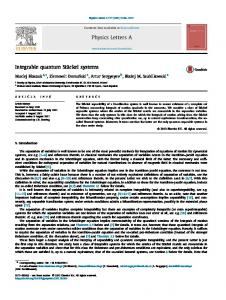
Employing now eqs. (1) and (3) for two initial states |αi (α = a, b) which share the same value of the energy density but not the same values of the other higher charges, and solving for them the Generalized Bethe Ansatz equation (23) for the corresponding pseudo-energy, one gets the infinite time average of : ψ †2 (x)ψ 2 (x) : as function of the dimensionless coupling constant γ of the Lieb-Liniger model, as shown in Fig. 2. In this figure it is also plotted, for comparison, the curve which corresponds to the thermal equilibrium value for this observable. Few comments are in order. At strong coupling, i.e. γ → ∞, all curves must go to zero for the emerging fermionic nature of the theory in this limit. Hence, the difference between the thermal and the Generalized Gibbs Ensemble averages themselves is hardly distinguishable in this region. However, at weak coupling, one observes a rather large spread of values for this observable, for the obvious reason that there are of course innumerable many ways to get out of equilibrium and the integrable theory keeps memory of it. In particular, one can always arrange the expectation values of the higher charges to produce a weak dependence on γ of this observable, as it is the case for instance of the state |bi. Similar computation can be repeated for other observables as well and detailed discussion will be presented in the forthcoming publication [20].

7

g2 5

a

4

3

2

eq

1

b 2

4

6

8

Γ

10

-1

FIG. 2: Infinite time averages of hα|(: ψ †2 ψ 2 :)|αi (α = a, b) for two different quench states |ai and |bi with the same energy density (here E/L = 17) versus the dimensionless coupling constant γ of the Lieb-Liniger model. The thermal equilibrium curve for the same energy density is the dashed one.