Information-theoretic approach for selection of spatial and temporal ...

MARINE ECOLOGY PROGRESS SERIES Mar Ecol Prog Ser

Vol. 253: 17–24, 2003

Published May 15

Information-theoretic approach for selection of spatial and temporal models of community organization E. Godínez-Domínguez1, 2,*, J. Freire1 1

Departamento de Biología Animal, Biología Vegetal y Ecología, Universidad de A Coruña, Campus da Zapateira s/n, A Coruña 15071, Spain

2

Centro de Ecología Costera, Centro Universitario de la Costa Sur, Universidad de Guadalajara, V. Gómez Farias 82, San Patricio-Melaque, Jalisco 48980, Mexico

ABSTRACT: The literature on the ecology of marine assemblages includes frequent examples of data analysis with no well-defined alternative hypotheses for the definition of environmental variables (independent matrix for multivariate methods). Alternative models, whereby spatial or temporal patterns are investigated, should be explicitly assumed. We present a parsimonious procedure for model selection in multivariate data combined with canonical correspondence analysis to determine the measure of explained variance for each tested model, using Akaike’s information criterion (AIC) for model selection. The AIC procedure is an effective tool for model selection and, in contrast to other conventional procedures that use only 1 implicit model and ignore other community patterns, it provides a framework for ranking hierarchical patterns that adds an alternative non-disjunctive perspective to assemblage analysis. Hierarchical patterns are revealed as layers in a scale-dependent framework. KEY WORDS: Akaike’s information criterion · Model selection · Spatial models · Temporal models · Canonical correspondence analysis · Parsimony · Marine benthic communities · Community dynamics Resale or republication not permitted without written consent of the publisher

Variability in abundance, distribution and diversity inevitably involves a hierarchy of spatial and temporal scales in ecological communities. The availability and quality of habitats vary between localities on scales ranging from centimeters to hundreds of kilometers, affecting abundance and diversity both directly and indirectly through modification of biotic interactions (Underwood et al. 2000). The identification of ecological assemblages at a particular place and time is a multivariate problem, where each species is considered a variable (Anderson & Clements 2000) that must be solved to determine the structural patterns of the community over environmental gradients. Most of the published literature on marine communities uses a purely descriptive observational approach, lacks a falsificationist approach and is unable

to reveal consistent patterns (see Underwood et al. 2000), thus limiting any conclusions. Although the designs of marine community surveys are becoming more rigorous with the development of sampling theory and the wide availability of software packages for multivariate analysis (e.g. Clarke & Warwick 1994, ˇ Legendre & Legendre 1998, ter Braak & Smilauer 1998), the main cause of the limitations in marine community studies is related to the lack of a procedure enabling selection of the best spatial and/or temporal model from a set of a priori models in a matrix of community data. Several examples in the scientific literature describe both spatial and temporal assemblage patterns using different statistical tests based on the relationships among different environmental variables and species abundance (or presence/absence). The most frequent flaws of these analyses are:

*Email: [email protected]

© Inter-Research 2003 · www.int-res.com

INTRODUCTION

18

Mar Ecol Prog Ser 253: 17–24, 2003

(1) The absence of an a priori explicit hypothesis. The only null hypothesis assumed in a typical direct gradient analysis is that the species data are unrelated to the environmental data (Jongman et al. 1995), and this is insufficient when a set of alternative models is not rigorously defined and tested. Examples of publications in which explicit hypotheses were tested are rare, and in most of the cases studies focus more on revealing relationships with some environmental variables (the more the better) than on falsifying a priori hypotheses. The prevailing method seems to ‘search for relations with environmental variables, and if you find a significant one, then endeavors to explain the ordination patterns and formulate hypotheses’. When an independent matrix is constructed, then implicitly (and probably unconsciously) a set of hypotheses is created to explain them. (2) Flaws in the selection of a priori hypotheses. Relationships between the environment and species are not consistently supported since in most cases the selected environmental variables do not represent essential processes (making it impossible to determine the right response variables necessary to define the dynamic environment) and provide an inadequate environmental context. Many of the environmental variables included in the analyses exhibit collinearity. (3) Ordination patterns emerge as spurious relationships or statistical artifacts, reflecting more the statistical procedures employed than ecological causality. The statistical methods invariably generate patterns from the species environment matrix relations that falsify the null hypothesis. In many cases they do not allow successful inferences about patterns and ecological processes to be drawn. (4) The arbitrary selection method. Different ordination and classification methods may give different results when used to model the same data set (Anderson & Clements 2000), indicating the need for a set of alternative assemblage models and a validation method. Models should be used as a key tool, ‘confronting hypotheses with data’ in a model validation strategy (Hilborn & Mangel 1997). Information-theoretic methods avoid the above problems. They comprise a statistical methodology for the definition and selection of an a priori set of alternative hypotheses (expressed as models), rather than a simple statistical test of a null hypothesis (Burnham & Anderson 1998, Anderson et al. 2000). This approach estimates the formal likelihood of each model and the rank of each hypothesis (a measure of precision that incorporates model selection uncertainty), and provides simple methods for integrating alternative models when making inferences (Anderson et al. 2000). Here we propose a procedure based on the information-theoretic approach that utilizes the output of uni-

modal methods of multivariate analysis (ter Braak & Sˇmilauer 1998) to analyze competing a priori models of the spatial and temporal organization of marine communities and to select the most parsimonious model. Parsimonious models achieve a proper tradeoff between bias and variance, and all model selection methods are based to some extent on the principle of parsimony (Burnham & Anderson 1998).

METHODS Procedure for model formulation and selection. The proposed procedure consists of 3 steps: (1) Definition of a set of a priori models: The definition of the universe of probable models would be ideal. However, usually the available data on the community concerned are insufficient to develop a solid set of hypotheses. A clear theoretical concept of the possible ecological patterns in the data set should be established using alternative models and reflected on the codification of the matrix of independent variables. Codification based on dummy variables (see ter Braak & Sˇmilauer 1998, Legendre & Anderson 1999, Anderson & Clements 2000) allows the construction of the matrices to reflect the expected grouping of sampling statistics in various alternative configurations of time, space and other experimental factors and their interactions. (2) Statistical fit of models to data: In the example presented in this paper, we used canonical correspondence analysis (CCA) (ter Braak & Sˇmilauer 1998) to measure the fit of the model to data by means of the trace of each tested model. Other analyses such as redundancy analysis or detrended CCA could be used to measure the information extracted to data. Direct gradient analysis is one of the methods most frequently used to assess assemblage variability and to test the statistical significance of the effect of environmental variables on community structure (ter Braak & Sˇmilauer 1998). Direct gradient analysis incorporates information about the environment into the analysis of multivariate species data (ter Braak 1994) and determines the main patterns in the relationships between species abundance and independent variables. One of the most common implementations of the direct gradient techniques is CCA (usually using the software CANOCO; ter Braak 1996), which selects the linear combinations of environmental variables that maximize the dispersion of the species scores. CCA combines the concepts of ordination and regression (Legendre & Legendre 1998), and data on species composition are represented by a Gaussian response model in which the explanatory variable is a linear combination of the environmental variables. The key

Godínez-Domínguez & Freire: Information-theoretic approach to model selection

assumption is that the response model is unimodal, even though CCA is extremely robust when this assumption does not hold (Jongman et al. 1995). The statistical significance of the relationship between the species matrix and the set of environmental variables is assessed in the CANOCO package using Monte Carlo permutation tests. The statistical test is an F-ratio of the sum of all canonical eigenvalues and the residual sum of squares (RSS). This test is highly sensitive to all manner of deviations from the null hypothesis (ter Braak & Sˇmilauer 1998), which assumes the non-significance of relationships between the a priori environmental variables and the species matrix. In other words, each permutation of the samples in the species data is equally likely. The design of the hypotheses to be tested using permutation tests involves the construction of a matrix with quantitative and/or binary environmental variables, or the definition of matrices of the analysis of variance type, where either single or several classification factors and their interactions are included and recorded as dummy variables (Legendre & Legendre 1998). A multivariate analog of the univariate RSS is: RSS = (sum of all eigenvalues) − ∑i =1 tracei h

19

between 2 models (Kullback 1959); it is also considered a discrepancy measure (Burnham & Anderson 1998). The true statistical sampling distribution of the data is established by ƒ(x) and the model by g(x|θ) (with a known form but generally unknown parameters, denoted by θ). The K-L discrepancy then is: l ( ƒ, g ) =

 ƒ( x ) 

∫ ƒ( x ) log  g ( x | θ)  dx

(2)

The K-L discrepancy is deeply rooted in information theory and is by no means an arbitrary choice of metric here. Essentially, l ( ƒ,g) is a unique metric to use in the context of maximum likelihood theory (Anderson et al. 1994). Akaike (1973) found a relationship between the K-L discrepancy and an expected log-likelihood, and this finding has allowed major practical and theoretical advances in model selection and the analysis of complex data sets (Burnham & Anderson 2001). The maximized log-likelihood is a biased estimator of this expected log-likelihood, and the asymptotic bias equals K, the number of free parameters in the model (Akaike 1973); hence, AIC = − 2 log [L(θˆ )] + 2K

(3)

(1)

where h is the number of factors in the model (Legendre & Anderson 1999). (3) Selection of the best model: The best model among competing multivariate models is determined by a parsimonious procedure called the Akaike information criterion (AIC). If we presume that in a direct gradient analysis each environmental variable extracts a fraction of the total variability in the data (including environmental variables constructed by a random process), a model that considers more variables (and therefore, in our case, more groups of sampling stations) has to extract more variability. In the extreme case, we could codify each sampling station as one separate group, in which case a CCA would approximate a correspondence analysis (CA) (ter Braak & Sˇmilauer 1998). The principle of parsimony is defined as the tradeoff between variance (uncertainty) and the number of estimable parameters (groups in an ordination model) in the model (Burnham & Anderson 1998). Akaike information criterion. Akaike (1973) introduced his entropy maximization principle as a theoretical basis for model selection and found a simple relationship between the Kullback-Liebler (K-L) distance (or information) and Fisher’s maximized log-likelihood function (Burnham & Anderson 1998). This relationship leads to a simple, effective and very general methodology for selecting a parsimonious model for the analysis of empirical data called the AIC. The K-L distance can be conceptualized as a direct distance

This has become known as Akaike’s information criterion, or AIC, and it enables the combination of estimation and model selection under the single theoretical framework of optimization (Anderson et al. 2000). A simple transformation of the estimated RSS allows the value of log [L(θˆ )] to be obtained using least-squares estimation with normally distributed errors rather than the likelihood method. For all standard linear models, we can take: log [L(θˆ )] = −

1 n log(σˆ 2 ) 2

(4)

where log = loge, n is sample size and σˆ 2 = RSS/n (Burnham & Anderson 1998). To avoid the bias in AIC estimates due to the relationship between number of parameters and sample size, Sugiura (1978) derived a secondary variant of AIC: 2K (K + 1)  AICc = AIC +   n − K − 1 

(5)

AICc (Aikaike information criterion corrected) is used when the ratio n/K < 40. As AICc is measured on a relative scale, Burnham & Anderson (1998) recommended the computation of the AIC (∆ i ) differences rather than the AIC values for all candidate models in the set: ∆ i = AICi – minAIC (6) Such differences estimate the expected relative K-L differences between ƒ and gi (x|θˆ ). In order to get a bet-

20

Mar Ecol Prog Ser 253: 17–24, 2003

ter measurement of the plausibility of each model as being the actual K-L model, Akaike (1983) proposed exp (–1⁄2 ∆i) as being the relative likelihood of the model. Burnham & Anderson (1998) normalized Eq. (6) to a set of positive Akaike weights (wi) summing 1: wi =

1 exp  − ∆ i   2  R

1 ∑ exp  − 2 ∆ r 

(7)

Model t1: community organization was similar on the cruises (DEM 1 = 2 = 3 = 4 = 5). Model t2: community organization is different in each cruise (DEM 1 ≠ 2 ≠ 3 ≠ 4 ≠ 5). Model t3: community organization changed seasonally according to the hydrographic structure: transition period ≠ tropical period ≠ subtropical-temperate period (DEM 1 and 4) ≠ (DEM 2 and 5) ≠ (DEM 3). Model t4 (constructed in accordance with the results of the selection of the spatial models): tran-

r =1

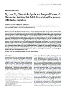
As ∆ i becomes larger, wi becomes smaller and it becomes increasingly less probable that Model i is the best K-L model based on the design and sample size used. Ecological example of the procedure. The data used for the application of the proposed procedure were from experimental fishing cruises with a shrimp trawler on in the inner continental shelf of the Mexican central Pacific (see Godínez-Domínguez & GonzálezSansón 1998 for details of the study area). The stratified experimental design was chosen to analyze spatial patterns of macroinvertebrate assemblages. Five cruises (named DEM 1 to 5) were conducted aboard the RV ‘BIP-V’ of the University of Guadalajara, Mexico, and covered the different hydroclimatic and fishing seasons. The main sea surface currents define 3 seasons: the California Current (CC) (the subtropicaltemperate affinity period), the North Equatorial Counter-Current (NCC) (the tropical affinity period), and a transition (the transition period) between these 2 currents in which neither dominates. Seven sites along the coast were sampled during each cruise at 4 depths (20, 40, 60 and 80 m at each site), making a total of 28 sampling stations per cruise. Two main sources of spatial variability in community structure are proposed as basic a priori hypotheses: depth and spatial variability along the coast due to the alternation of sheltered and exposed areas. A set of possible models describing the spatial organization of the community was defined (Models s1 to s8; Fig. 1). The models reflect the existence of effects on community organization of the depth gradient, exposure level and the interaction of both these factors. The interaction between these 2 factors was included to examine the possibility that only in shallow waters was the effect of exposure (through waves, tides and input of freshwater) critical. The selection of a spatial model was carried out independently for each cruise. For the temporal analysis, several alternative models were tested, from the absence of seasonality to a seasonal pattern determined by the main hydroclimatic coastal processes. Temporal patterns in species assemblages were analyzed using a matrix that included data from all cruises, and no spatial structure was included in these models. The models had the following designs:

Fig. 1. Schematic representation of the different models of spatial community organization based on 3 basic hypotheses: (1) Effect of depth gradient; 3 levels of effects are proposed: (i) no effect; (ii) differences among all the depth strata; (iii) differences between the shallow (20 and 40 m) and deep (60 and 80 m) strata (previous data indicated an important ecological discontinuity between 40 and 60 m; Godínez-Domínguez et al. unpubl data). (2) Degree of exposure (alongshore variability), with 2 levels of effects: (i) no effect; (ii) differences between exposed and sheltered areas. (3) Interaction between depth and exposure; some models include possibility that exposure is only effective in shallow waters. In the diagram, each box represents samples with homogeneous community structure

Godínez-Domínguez & Freire: Information-theoretic approach to model selection

21

sition period ≠ tropical period + subtropical-temperate period (DEM 1 and 4) ≠ (DEM 2, 5 and 3). CCAs with non-transformed species abundance data (organisms ha–1) were performed for each cruise, carrying out a run for each spatial model tested and introducing a dummy variable coded file as environmental matrix. File codifications (Fig. 2, Table 1) should include 1 nominal variable for each box in the model (sample group with homogeneous community structure). This codification scheme produces a last class or category that is always collinear with the preceding classes; however this does not affect the ordination results (ter Braak & Sˇmilauer 1998). The sum of all unconstrained eigenvalues and the sum of all canonical eigenvalues are used to estimate the RSS. The number of variables coded or groups in the model tested were considered as the number of parameters, K, in the estimation of the AIC. Fig. 2. Study area and sampling stations (Stns 1 to 28)

RESULTS AND DISCUSSION Table 1. Environmental characteristics (depth and degree of exposure) of sampling stations, and examples of the codification scheme used to represent the spatial models (here Models s1 and s6 are shown as contrasting examples). Environmental variables are dummy variables that define each group of sampling stations (boxes in Fig. 1) with homogeneous community structure. Sh: sheltered; Ex: exposed Stn

1 2 3 4 5 6 7 8 9 10 11 12 13 14 15 16 17 18 19 20 21 22 23 24 25 26 27 28

Spatial features Depth Exposure

20 40 60 80 20 40 60 80 20 40 60 80 20 40 60 80 20 40 60 80 20 40 60 80 20 40 60 80

Ex Ex Ex Ex Sh Sh Sh Sh Sh Sh Sh Sh Ex Ex Ex Ex Sh Sh Sh Sh Ex Ex Ex Ex Ex Ex Ex Ex

Model s1 Sh Ex

0 0 0 0 1 1 1 1 1 1 1 1 0 0 0 0 1 1 1 1 0 0 0 0 0 0 0 0

1 1 1 1 0 0 0 0 0 0 0 0 1 1 1 1 0 0 0 0 1 1 1 1 1 1 1 1

20 and 60 m 40 m Sh 1 1 0 0 1 1 0 0 1 1 0 0 1 1 0 0 1 1 0 0 1 1 0 0 1 1 0 0

0 0 0 0 0 0 1 0 0 0 1 0 0 0 0 0 0 0 1 0 0 0 0 0 0 0 0 0

Model s6 80 m 60 m Sh Ex 0 0 0 0 0 0 0 1 0 0 0 1 0 0 0 0 0 0 0 1 0 0 0 0 0 0 0 0

0 0 1 0 0 0 0 0 0 0 0 0 0 0 1 0 0 0 0 0 0 0 1 0 0 0 1 0

80 m Ex 0 0 0 1 0 0 0 0 0 0 0 0 0 0 0 1 0 0 0 0 0 0 0 1 0 0 0 1

The permutation tests (Table 2) show that it is possible for the same species data set to obtain a significant fit to several spatial models, and that in several cases the ecological support of some of these models can vary substantially. Thus, an alternative objective criterion for model selection appears to be necessary. AIC results (Table 3) indicated that during Cruises DEM 1 and 4 (hydroclimatic transition period) the best model was s2 (effect of depth differentiating shallow and depth strata), and during Cruises DEM 2, 5 (tropical period) and 3 (subtropicaltemplate period), s5 (differentiating 4 depth strata) was the best model. Effect of exposure was not included in any of the models selected. For Cruise DEM 1, Models s2 to s8 were statistically significant (permutation tests, p < 0.05); Models s2 to s8 were statistically significant (permutation tests, p < 0.05). Models s3 and s4, which included an interaction between depth and exposure, were ranked 2nd and 4th respectively. Statistically all the tested models showed a significant fit except Model s1. For Cruises DEM 2 and 3, all the tested models were significant (except Model s1 for DEM 2 and

22

Mar Ecol Prog Ser 253: 17–24, 2003

Table 2. Results of permutation tests of canonical correspondence analysis (CCA) to determine significance of relationship between species and fitted spatial models Cruise

DEM 1 Total inertia Trace p-value, first canonical axis p-value, global test DEM 2 Total inertia Trace p-value, first canonical axis p-value, global test DEM 3 Total inertia Trace p-value, first canonical axis p-value, global test DEM 4 Total inertia Trace p-value, first canonical axis p-value, global test DEM 5 Total inertia Trace p-value, first canonical axis p-value, global test

Spatial Model s4 s5

s1

s2

s3

2.857 0.065

2.857 0.652

0.814

0.001

2.857 0.821 0.001 0.001

2.857 0.865 0.001 0.001

4.556 0.284

4.556 0.497

0.529

0.001

4.556 0.797 0.006 0.001

4.812 0.204

4.812 0.489

0.333

0.001

2.550 0.047

2.550 0.082

0.774

0.082

4.455 0.036

4.455 0.213

0.986

0.225

Model s6 for DEM 3). All DEM 4 spatial models tested were not significant, and for Cruise DEM 5 a significant fit was obtained for Model s5. Spatial hierarchical patterns in the assemblage distribution are evident from our results. With the procedure proposed, it is possible not only to determine the best model but to rank the different hypotheses according to parsimonious criteria, avoiding the current trend to determine only 1 spatial model which is inferred in most cases from the graphical CCA output display. AIC is useful not only as an effective selection model tool, but also to rank hierarchical spatial patterns, which add an alternative non-disjunctive perspective to assemblage analysis, in contrast to other conventional procedures that use only 1 implicit model and ignore other hierarchical patterns in a community. This is illustrated by Cruises DEM 1, 2, and 3, for which a wide range of models adequately fit the data (Models s2 to s8): any of these models can be presented as a ‘true model’ if a selection procedure is not applied. The analysis of temporal models showed that the more complex model (Model t2) (according to the number of parameters) was the best model based on the AIC procedure (Table 4). This indicates that community structure was different for each cruise, with no grouping by hydroclimatic similarity, despite the fact

s6

s7

s8

2.857 0.979 0.001 0.001

2.857 1.058 0.001 0.001

2.857 1.242 0.001 0.001

2.857 1.408 0.001 0.001

4.556 1.081 0.011 0.002

4.556 1.503 0.001 0.001

4.556 1.094 0.043 0.023

4.556 1.940 0.001 0.001

4.556 2.444 0.001 0.001

4.812 0.657 0.006 0.009

4.812 0.890 0.004 0.008

4.812 1.251 0.001 0.001

4.812 0.955 0.150 0.128

4.812 1.520 0.010 0.007

4.812 2.046 0.108 0.006

2.550 0.119 0.560 0.620

2.550 0.155 0.790 0.830

2.550 0.419 0.050 0.077

2.550 0.514 0.163 0.179

2.550 0.590 0.190 0.140

2.550 0.653 0.324 0.437

4.455 0.225 0.530 0.742

4.455 0.367 0.394 0.704

4.455 0.981 0.001 0.003

4.455 0.402 0.858 0.852

4.455 1.157 0.001 0.053

4.455 1.479 0.011 0.140

that some cruises had the same spatial structure. Model t3, which grouped cruises by hydroclimatic seasons, was statistically significant, and was ranked third according to its AIC value after Models t2 and t4 (similar community structure in all cruises). Permutation tests of the CCA (Table 5) showed that Models t2 and t3 were both statistically significant (p < 0.05), although both indicated contrasting patterns of community organization (similarity among cruises vs grouping by hydroclimatic season). The hierarchical spatial structure was determined by the relationship between the 2 main physiographic traits of a coastal shelf-depth and exposure gradients. The selected models illustrate how the AIC methods apply the parsimony principle, leading to a model that incorporates the smallest possible number of parameters required for adequate representation of the data. Following this principle the ‘true model’ achieves a successful tradeoff between bias and variance (Burnham & Anderson 1998). Development of an a priori set of candidate models should include a global model, i.e. a model that has many parameters and includes all potentially relevant effects (in our case Model s8). Models with fewer parameters can then be derived by modifications to the global model (Burnham & Anderson 1998).

23

Godínez-Domínguez & Freire: Information-theoretic approach to model selection

Table 3. Results of procedure applied for selection of spatial models using Akaike information criterion. Shaded columns indicate most parsimonious model. n = 28 sampling stations on all cruises. RSS: residual sum of squares; AICc: Akaike information criterion corrected; w: Akaike weights Cruise s1

s2

Spatial Model s4 s5

s3

s6

s7

s8

DEM 1 Total inertia Trace RSS/n AICc w

2.857 0.065 0.100 –60.072 0.011

2.857 0.652 0.079 –66.681 0.291

2.857 0.821 0.073 –66.394 0.252

2.857 0.865 0.071 –64.267 0.087

2.857 0.979 0.067 –65.917 0.199

2.857 1.058 0.064 –64.132 0.081

2.857 1.242 0.058 –63.880 0.072

2.857 1.408 0.052 –59.338 0.007

DEM 2 Total inertia Trace RSS/n AICc w

4.556 0.284 0.153 –48.163 0.053

4.556 0.497 0.145 –49.596 0.109

4.556 0.797 0.134 –49.225 0.091

4.556 1.081 0.124 –48.686 0.069

4.556 1.503 0.109 –52.311 0.425

4.556 1.094 0.124 –45.803 0.016

4.556 1.940 0.093 –50.376 0.162

4.556 2.444 0.075 –48.789 0.073

DEM 3 Total inertia Trace RSS/n AICc w

4.812 0.204 0.165 –46.043 0.116

4.812 0.489 0.154 –47.831 0.283

4.812 0.657 0.148 –46.421 0.140

4.812 0.890 0.140 –45.298 0.080

4.812 1.251 0.127 –48.001 0.308

4.812 0.955 0.138 –42.778 0.023

4.812 1.520 0.118 –43.940 0.040

4.812 2.046 0.099 –41.236 0.010

DEM 4 Total inertia Trace RSS/n AICc w

2.550 0.047 0.089 –63.132 0.259

2.550 0.082 0.088 –63.526 0.316

2.550 0.119 0.087 –61.429 0.111

2.550 0.155 0.086 –59.108 0.035

2.550 0.419 0.076 –62.378 0.178

2.550 0.514 0.073 –60.667 0.076

2.550 0.590 0.070 –58.459 0.025

2.550 0.653 0.068 –51.795 0.001

DEM 5 Total inertia Trace RSS/n AICc w

4.455 0.036 0.158 –47.216 0.170

4.455 0.213 0.152 –48.361 0.302

4.455 4.455 0.225 0.367 0.151 0.146 –45.92000 –44.137 0.089 0.037

4.455 0.981 0.124 –48.694 0.357

4.455 0.402 0.145 –41.390 0.009

4.455 1.157 0.118 –43.889 0.032

4.455 1.479 0.106 –39.187 0.003

K (no. of parameters)

2

2

Table 4. Results of procedure applied for selection of temporal models using Akaike information criterion (K: no. of parameters; n: sample size; AICc: Akaike information criterion corrected; RSS: residual sum of squares; w : Akaike weights) Parameter 000t1 K n Total inertia Trace RSS/n AICc w

0001 000140 0006.218 0000.000 0000.044 –433.958 0000.226

Temporal Model 000t3 000t3 0003 000140 0006.218 0000.180 0000.043 –433.923 0000.222

0005 000140 0006.218 0000.410 0000.041 –435.089 0000.397

3

4

4

5

6

8

Table 5. Results of permutation tests of canonical correspondence analysis (CCA) to determine significance of relationship between species and fitted temporal models. CCA of Temporal Model t1 was not carried out because this model assumes an ordination of only 1 group and the trace should approximate zero

000t4 0002 000140 0006.218 0000.058 0000.044 –433.212 0000.155

According to the AIC values for each cruise, depth is the most recognizable gradient in the spatial distribution of macrofaunal assemblages. The main bathymetric discontinuity lies between 40 and 60 m. Degree of exposure constitutes a secondary gradient, and is

t2 Total inertia Trace p-value first canonical axis p-value global test

Temporal Model t3 t4

6.218 0.410 0.001 0.001

6.218 0.180 0.008 0.013

6.218 0.058 0.165

only relevant for shallow waters. The main problem of conventional analyses is that they can introduce bias toward the most obvious gradients, while other less evident, but potentially important sources of variation can remain undetected. Using the AIC procedure, hierarchical patterns appear as layers in a scaledependent resolution framework.

Mar Ecol Prog Ser 253: 17–24, 2003

24

Acknowledgements. This research was partially funded by the University of Guadalajara, Mexico, by the Consejo Nacional de Ciencia y Tecnología (CONACyT), Mexico, and by Grant REN2000-0446 from the Ministerio de Ciencia y Tecnología, Spain.

Akaike H (1973) Information theory as an extension of the maximum likelihood principle. In: Petrov BN, Csaki F (eds) 2nd International Symposium on Information Theory. Akademiai Kiado, Budapest, p 267–281 Akaike H (1983) Information measures and model selection. International Statistical Institute, Voorburg Anderson DR, Burnham KP, White GC (1994) AIC model selection in overdispersed capture-recapture data. Ecology 75:1780–1793 Anderson DR, Burnham KP, Thompson WL (2000) Null hypothesis testing: problems prevalence, and an alternative. J Wildl Manage 64:912–923 Anderson MJ, Clements A (2000) Resolving environmental disputes: a statistical method for choosing among competing cluster models. Ecol Appl 10:1341–1355 Burnham KP, Anderson DR (1998) Model selection and inference. A practical information-theoretic approach. Springer-Verlag, New York Burnham KP, Anderson DR (2001) Kullback-Leibler information as a basis for strong inference in ecological studies. Wildl Res 28:111–119 Clarke KR, Warwick RM (1994) Change in marine communities — an approach to statistical analysis and interpretation. Plymouth Marine Laboratory, Plymouth

Godínez-Domínguez E, González-Sansón G (1998) Variación de los patrones de distribución batimétrica de la fauna macrobentónica en la plataforma continental de Jalisco y Colima, México. Cienc Mar 24:337–351 Hilborn R, Mangel M (1997) The ecological detective; confronting models with data. Princeton University Press, Princeton Jongman RH, ter Braak CJF, van Tongeren OFR (1995) Data analysis in community and landscape ecology. Cambridge University Press, Cambridge Kullback S (1959) Information theory and statistics. John Wiley & Sons, New York Legendre P, Anderson MJ (1999) Distance-based redundancy analysis: testing multispecies responses in multifactorial ecological experiments. Ecol Monogr 69:1–24 Legendre P, Legendre L (1998) Numerical ecology, 2nd edn. Elsevier, Amsterdam Sugiura N (1978) Further analysis of the data by Akaike’s information criterion and the finite corrections. Commun Statist Theory Meth 7:13–26 ter Braak CJF (1994) Canonical community ordination. Part I: Basic theory and linear methods. Ecoscience 1:127–140 ter Braak CJF (1996) Unimodal models to relate species to environment. DLO-Agricultural Mathematics Group, Wageningen ter Braak CJF, Sˇmilauer P (1998) CANOCO reference manual and user’s guide to Canoco for Windows; software for canonical community ordination (Version 4.0). Microcomputer Power, Ithaca, NY Underwood AJ, Chapman MG, Connell SD (2000) Observations in ecology: you can’t make progress on processes without understanding the patterns. J Exp Mar Biol 250: 97–115

Editorial responsibility: Otto Kinne (Editor), Oldendorf/Luhe, Germany

Submitted: May 27, 2002; Accepted: November 1, 2002 Proofs received from author(s): April 23, 2003

LITERATURE CITED