Aug 27, 2010 - Thomas Hélie (1), Thomas Hézard (1), Rémi Mignot (1-2) ... With this intention, a refined version of the "Webster" horn equation is considered, ...
Proceedings of 20th International Congress on Acoustics, ICA 2010 23–27 August 2010, Sydney, Australia
Input impedance computation for wind instruments based upon the Webster-Lokshin model with curvilinear abscissa Thomas Hélie (1), Thomas Hézard (1), Rémi Mignot (1-2) (1) Equipe Analyse/Synthèse, CNRS UMR 9912 - IRCAM, 1 place Igor Stravinsky, 75004 Paris, France (2) Institut Langevin, ESPCI ParisTech, 10 rue Vauquelin, 75005 Paris, France. PACS: 43.20.Mv, 43.75.Fg, 43.75.Ef. ABSTRACT This work addresses the computation of acoustics immittances of axisymmetric waveguides, the shape of which is C1-regular (i.e. continuous and with a continuous derivative with respect to the space variable). With this intention, a refined version of the "Webster" horn equation is considered, namely, the "Webster-Lokshin equation with curvilinear abscissa", as well as simplified models of mouthpieces and well-suited radiation impedances. The geometric assumptions used to derive this uni-dimensional model (quasi-sphericity of isobars near the wall) are weaker than the usual ones (plane waves, spherical waves or fixed wavefronts). Moreover, visco-thermal losses at the wall are taken into account. For this model, exact solutions of the acoustic waves can be derived in the Laplace or the Fourier’s domains for a family of parametrized shapes. An overall C1-regular bore can be described by connecting such pieces of shapes under the constrain that junctions are C1-regular. In this case and if the length of the bore is fixed, a description with N pieces precisely has 2N+1 degrees of freedom. An algorithm which optimizes those parameters to obtain a target shape has been built. It yields accurate C1-regular descriptions of the target even with a few number of pieces. A standard formalism based on acoustic transfer matrices (deduced from the exact acoustic solutions) and their products make the computation of the input impedance, the transmittance (and other immittances) possible. This yields accurate analytic acoustic representations described with a few parameters. The paper is organized as follows. First, some recalls on the history of the "Webster" horn equation and of the modeling of visco-thermal losses at the wall are given. The "Webster-Lokshin model" under consideration is established. Second, the family of parametrized shapes is detailed and the associated acoustic transfer matrices are given. Third, the algorithm which estimates the optimal parameters of the C1-regular model of target shapes is presented. Finally, input impedances obtained using this algorithm (and the Webster-Lokshin model) are compared to measured impedances (e.g. that of a trombone) and to results of other methods based on the concatenation of straight or conical pipes. This paper is the French to English translation and corrected version of [Hélie, Hézard, and Mignot 2010].
1. ON THE WAVE EQUATION IN HORNS 1.1. History summary and context Uni-dimensional models and geometry The first unidimensional model of the acoustic propagation in axisymmetric pipes is due to [Lagrange 1760-1761] and [Bernoulli 1764]. This equation, usually called “horn equation” or “Webster equation” [Webster 1919] has been extensively investigated [Eisner 1967] and is based on hypotheses which have been periodically revised. So, to preserve the orthogonality of the rigid motionless wall and wavefronts, [Lambert 1954] and [Weibel 1955] contest derivations based planar waves and postulate spherical ones. The quasi-sphericity was experimentally confirmed for a horn profile in the low frequency range by Benade and Janson [Benade and Jansson 1974]. Later, Putland [Putland 1993] pointed out that every one-parameter acoustic fields obey a Webster equation for particular coordinates and that only planar, cylindrical and spherical waves could correspond to such coordinates.
ICA 2010
Though this limitation, some refined uni-dimensional models have still been looked for because of their simplicity: they make the computation of impedances easy and the frequency range that is not perturbed by transverse modes [Pagneux, Amir, and Kergomard 1996] is large for many wind musical instruments. Thus, [Agulló, Barjau, and Keefe 1999] assumes ellipsoidal wavefronts. In [Hélie 2003], an exact model is derived for coordinates that rectify isobars and a Webster equation is deduced under the assumption that isobars are quasi-spherical (at order 2) near the wall (assumption that is considered in this paper). Generalizations based upon Webster’s horn equation have been also studied in [Martin 2004].
Visco-thermal losses A second model refinement concerns the modeling of visco-thermal losses at the wall. First, Kirchhoff has introduced thermal conduction effects, extended the Stoke’s theory and derived some basic solutions in the free space and in a pipe. Moreover, he gave the exact general dispersion relation for a cylinder if/whether the problem is ax-
1
23–27 August 2010, Sydney, Australia
Proceedings of 20th International Congress on Acoustics, ICA 2010
isymmetric [Kirchhoff 1868] (a generalized formula for non symmetric versions is given in [Bruneau et al. 1989, eq. (56)]).
nential wave). In the modal case, the following geometric invariant identity is deduced from the isobar wave equation
Some simplified modelings have also been proposed. Zwikker and Kosten (cf. e.g. [Chaigne and Kergomard 2008, p210]) have introduced models in which effects due the viscous and the thermal boundary layers were separated. The validity conditions for this theory can be found in [Kergomard 1981; Kergomard 1985] which exhibit more immediate links between this model and the Kirchhoff dispersion relation. Cremer has derived the equivalent admittance for plane waves which are reflected on a plane baffle w.r.t. their incidence angle [Cremer 1948]. This result coincides with that of Kirchhoff for rectangular waveguides which are large enough, that is, for which the boundary layer thickness is much lower than the rectangle characteristic lengths.
� � � � (∂s f )2 + (∂s g)2 + 2 (∂s f )2 + (∂s g)2 s k02 = 0, ∂s ln g2 2 2 (∂u f ) + (∂u g)
For these simplified models, the wave equations include a damping term that involves a fractional time derivative (see the Lokshin equation [Lokshin 1978; Lokshin and Rok 1978] and also [Polack 1991]). Exact solutions of the Lokshin equation have been derived in [Matignon 1994; Matignon and Novel 1995] which exhibit long memory effect. A Webster equation which includes such a damping term has been established in [Hélie 2003].
Context and approach In this paper, the acoustic model is derived assuming that isobars are quasi-spherical near the wall and describing the visco-thermal losses by the Cremer wall admittance. The main steps of its derivation are recalled below. 1.2. Wave equation and isobars Consider the cylindrical coordinate system (r, θ , z) and suppose the problem to be axisymmetric with respect to axis (Oz). Isobars can be locally described by r = f (s, u,t), z = g(s, u,t), θ ∈ [0, 2π [, where s indexes isobars and u is a (non-collinear) free coordinate. Since the pressure depends on s but not u, the time-varying maps described by ( f , g) are such that ∃p P(z = f (s, u,t), r = g(s, u,t), t) = p(s,t).
Using this property and the � change of coordinates � (z, r,t) → (s, u,t), the wave equation ∂z2 + 1r ∂r + ∂r2 − c12 ∂t2 P(z, r,t) = 0 rewrites � 1 � α (s,u,t)∂s2 + β (s,u,t)∂s + γ (s,u,t)∂s ∂t + 2 ∂t2 p(s,t)=0, (1) c
where α , β , γ are functions of f , g and of their derivatives with respect to s, u, t until order 2 (see [Hélie 2002; Hélie 2003] for the detailed formula). Applying operators ∂uk for k = 1, 2, 3 to the latter equation yields, for all s, u,t, ∂u α ∂u β ∂u γ 0 ∂s2 p 2 2 2 ∂u α ∂u β ∂u γ ∂s p = 0 . 0 ∂s ∂t p ∂u3 α ∂u3 β ∂u3 γ Hence, the determinant of the 3×3 matrix is zero. This gives a (purely geometric) necessary condition that every isobar map associated to an acoustic propagation must satisfy. In the time invariant case (∂t f = ∂t g=0), a similar study shows that the only admissible maps corresponds to the well-known cases, namely, plane waves, cylindrical waves, spherical waves and modes associated to a wavenumber that is either real (infinite oscillation) or complex imaginary (non oscillating expo-
2
if s is chosen as the level of the eigenfunction associated to the mode (see [Hélie 2003] for more details). As a consequence, no fixed map can describe a non modal 1D propagation if the pipe is neither straight, neither conical. 1.3. Ideal wall and 1D approximation An ideally rigid lossless and motionless wall coincides with a “pressure field line/tube” (see [Hélie 2002, p33] for degenerated cases). Choosing u orthogonal to s, there exists then ( f , g) and w such that f (s, u = w,t)= F(s), g(s, u = w,t)= R(s) where F, R is profile description of the pipe. At u = w,� coefficients in (1) are given by α (s, w,t) = 1/ F ′ (s)2 + R′ (s)2 , β (s, w,t) = 0 and � � d γ (s, w,t) R(s) ln ′ + ∂s ln ∂u g(s, u = w,t) . = α (s, w,t) ds F (s)
(2)
The only missing geometric information that is necessary to obtain a 1D model from (1) is in the second term of (2) which involves a first order partial derivative with respect to u (first order variation of the pressure field lines when moving away from the wall). To be compatible with the fact that isobars must be (i) planes in straight pipes, (ii) spherical in cones, (iii) orthogonal to the wall, (iv) quasi-spherical in horns [Benade and Jansson 1974], (v) dependent on the time, the following assumption is considered: near the wall, isobars slowly deviate from its tangent spherical approximation. More precisely, the relative deviation (denoted ζ (s, u,t)) (see [Hélie 2002]) satisfies ∂uk ζ (s,u=w,t) = 0 for k = 0 (contact) and k = 1 (tangency). Assuming the availability for k = 2 (deviation slower than a parabola), it follows γ (s,w,t) R′ (s) that α (s,w,t) = 2 R(s) . This leads to the Webster equation �
∂ℓ2 + 2
R′ (ℓ) 1 � ∂ℓ − 2 ∂t2 p(ℓ,t) = 0, R(ℓ) c
(3)
if s = ℓ is chosen as the curvilinear abscissa which measures the length of the wall profile (α (s,u=w,t) = 1). 1.4. Cremer wall admittance When visco-thermal boundary layers appear at the wall (/// are present), isobars are no more orthogonal to the wall. If the thickness of the boundary layers is lower than R(ℓ) and the curvature radius of the profile, this perturbation can be approximated through the Cremer wall admittance [Cremer 1948]. Assuming that isobars and their tangent spherical approximations still locally coincide at order 2, a perturbed version of (3) is obtained [Hélie 2002; Hélie 2003]. It is given by �
∂ℓ2 + 2
R′ (ℓ) 1 2ε (ℓ) 3 � ∂ℓ − 2 ∂t2 − 3 ∂t 2 p(ℓ,t) = 0, R(ℓ) c c2
(4)
3
is a fractional time derivative [Matignon 1994] and where ∂t 2 √ 1−R′ (ℓ)2 ε (ℓ) = κ0 R(ℓ) quantifies the visco-thermal effects (κ0 = p √ ′ lv +(γ −1) lh ≈ 3×10⁻⁴ m1/2 in the air). This equation is sometimes called the “Webster (case ε = 0)-Lokshin (case R′ = 0)” equation.
ICA 2010
Proceedings of 20th International Congress on Acoustics, ICA 2010
1.5. Model under consideration, properties, validity In the sequel, we consider the propagation in the space of rectified isobars, assuming their quasi-sphericity at order 2 near the wall, including the damping effect due to visco-thermal losses at the wall, that is governed by the following equations �
∂ℓ2 −
i�� h1 � 2ε (ℓ) 3 ∂t2 + 3 ∂t 2 + ϒ(ℓ) R(ℓ) p(ℓ,t) = 0 (5) 2 c c2 ρ ∂t v(ℓ,t) + ∂ℓ p(ℓ,t) = 0 (6)
ϒ = R′′ /R.
where If R is twice differentiable, then (5) is equivalent to (4). Outside the boundary layers, the particle velocity is collinear to the pressure gradient and it satisfies the Euler equation from which (6) is deduced after projection.
Properties of the change of coordinates z → ℓ Let z 7→ r(z) describe a pipe profile.p The profile length that is meaRz 1 + r′ (z)2 dz so that R(ℓ) = sured from 0 to z is L(z) = 0 � r L−1 (ℓ) . Then, differentiating R(L(z)) = r(z) leads to q R′ (L(z)) = r′ (z)/ 1 + r′ (z)2 .
Hence, the following two properties hold (i) |R′ (ℓ)| ≤ 1; (ii) R′ (ℓ) = 1 corresponds to a vertical slope. These geometric properties are quite unusual for the Webster model. Moreover, notice that (3-6) lead to the equations governing plane waves for a straight pipe (R′ /R = 0, ℓ = z), and spherical waves for cones (2R′ /R = 2/ℓ), as expected. If a profile z 7→ r(z) has a vertical slope at one extremity, the propagation model operates a natural connection with spherical waves.
Validity The lossless model (3) is exact if ϒ = 0. It provides accurate approximations if |ϒ| corresponds to a sufficiently small perturbation or if the frequency range is sufficiently low (see [Rienstra 2005] for a detailed analysis). Basically, the 1D assumption requires that there are no transverse modes in the pipes, that can be characterized by f < K + (Rmax )−1 with K + =
1.84 c ≈ 631.8 m.s−1 . 2π
The losses model is accurate if the thickness of the boundary layers is lower than the radius R and the curvature radius Rc √ ′ 2 3 1−R (ℓ) (1+R′ (z)2 ) 2 1 if s = z and by if s = ℓ. The given by ′′ R (z) R′′ (ℓ) most constraining condition is due to the viscous boundary layer. It is given by (see e.g. [Chaigne and Kergomard 2008, p212]) f > K − (Rmin )−2 with K − =
µ ≈ 2.39 × 10⁻⁶ m2 .s−1 . 2πρ
23–27 August 2010, Sydney, Australia
tions (5-6) become ��� � � �n � s �3 o s 2 2 2 +ϒ(ℓ) −∂ℓ R(ℓ)P(ℓ, s) = 0, +2ε (ℓ) c c U(ℓ, s) + ∂ℓ P(ℓ, s) = 0, ρs S(ℓ)
(7) (8)
where U(ℓ, s) = S(ℓ)V (ℓ) with S(ℓ) = π R(ℓ)2 . Closed-form analytical solutions can be derived if ε and ϒ are constant. Since R′′ (ℓ)−ϒ(ℓ)R(ℓ)=0, profiles associated with constant ϒ are such that ((A, B) ∈ R2 ) √ √ if ϒ < 0, R(ℓ) = A cos( −ϒℓ) + B sin( −ϒℓ), R(ℓ) = A + Bℓ, si ϒ = 0, √ √ if ϒ > 0. R(ℓ) = A cosh( ϒℓ) + B sinh( ϒℓ), These three families can be described by the unified formula R(ℓ) = ACϒ (ℓ) + B Sϒ (ℓ) , (9) � � 2 where (ϒ, ℓ)7→Cϒ (ℓ)= φ1 ϒ ℓ and (ϒ, ℓ)7→ Sϒ (ℓ)=ℓ φ2 ϒ ℓ2 are infinite differentiable function which are built from the following analytic functions (over C)
φ1 : z 7→ φ2 : z 7→
+∞
∑ (2k)!
zk
�
√ � = cosh z ,
zk ∑ (2k + 1)! k=0
�
=
k=0 +∞
√ � sinh z for z 6= 0 . √ z
Except the case where R is constant, these profiles do not correspond to constant ε . Then, for a sufficiently short interval [0, L], we chose to approximate ε by its mean value ε (ℓ) ≈ 1 RL L 0 ε (ℓ) dℓ. This defines what we call “piece of pipe” whose geometry is described by 4 parameters {A, B, ϒ, L} and inside which the propagation is characterized by the 3 constants ϒ, ε and c.
Acoustic transfer matrix of a piece of pipe Denoting � �T Xℓ (s) = P(ℓ, s) , U(ℓ, s) , solving (7-8) for coefficients ϒ and ε that are constant on [a,b] leads to Xb (s) = Tb,a (s) Xa (s), R(a) π R(b) � ρs � L , ρ s Mb,a (s)diag L , π R(a) is where Tb,a (s) = diag R(b) a matrix with a unitary determinant, which is given by � � � Mb,a (s) 11 = [1 , σa ] ∆ LΓ(s) , � � � Mb,a (s) 12 = [0 , −1] ∆ LΓ(s) , i h � � � Mb,a (s) 21 = σb −σa , σa σb − (LΓ(s))2 ∆ LΓ(s) , � � � Mb,a (s) 22 = [1 , −σb ] ∆ LΓ(s) ,
where ∆(z) = [cosh z , (sinh z)/z]T, where Γ(s) is a square-root �2 �3 of cs + 2ε cs 2 + ϒ, and the dimensionless quantity σℓ = R′ (ℓ) R(ℓ)/L
can be interpreted as a ratio of slopes.
2.2. C 1 -regular junctions of pieces of pipes
2. EXACT SOLUTIONS FOR PARAMETRIZED GEOMETRIES 2.1. Propagation model with constant coefficients Admissible profiles and regularity property In the Laplace domain (variable s) and for zero initial conditions, equa1
Remark: it can be checked that ε (ℓ) = κ0 Rc (ℓ)ϒ(ℓ) (if ϒ 6= 0).
ICA 2010
Cascade of pieces of pipes and geometric regularity constraints Consider the junction of N pieces of pipes with length Ln (this parameter is chosen to be let free). The complete profile depends on 4N parameters {An , Bn , ϒn , Ln}n∈[1,N] and is described by N
R(ℓ) =
∑ Rn (ℓ)1[ℓ
n−1 ,ℓn [
n=1
(ℓ) ,
∀ℓ ∈ [ℓ0 , ℓN ]
(10)
3
23–27 August 2010, Sydney, Australia
Proceedings of 20th International Congress on Acoustics, ICA 2010
where Rn (ℓ)=An Cϒn (ℓ)+Bn Sϒn (ℓ), {ℓn = ∑nk=1 Ln }0≤n≤N and ℓ1 , . . . ℓN−1 are the abscissa of the junction points. Writing the C 1 -regular constraint at the N − 1 junctions leads to the following 2(N − 1) equality constraints: � Rn (ℓn ) = Rn+1 (ℓn ), ∀n ∈ [1, N − 1] , (11) R′n (ℓn ) = R′n+1 (ℓn ). Notice that R is linear with respect to parameters An and Bn . The equation set is a linear system of dimension 2(N − 1) and 2N parameters {An , Bn }1≤n≤N . Choosing {A1 , B1 } as the 2 degrees of freedom (DOF), solving the system leads to solutions given by (see. [Hézard 2009]) [An , Bn ]T = Qn [A1 , B1 ]T ,
for 2 ≤ n ≤ N.
The number of DOF for such a profile described by N pieces of pipes is then 4N−2(N− 1) = 2N+2. According to the choices made above, the free parameters are A1 , B1 and {ϒn , Ln }1≤n≤N . Global acoustic transfer matrix from the acoustic point of view, connecting two pieces of pipes is achieved by imposing the continuity of the acoustic state Xℓ at junctions. This continuity makes sense at least when2 the junctions of profiles are C 1 -regular. Iterating this process to connect a sequence of pieces of pipes yields XℓN (s) TℓN ,ℓ0
= =
TℓN ,ℓ0 (s) Xℓ0 (s), TℓN ,ℓN−1 TℓN−1 ,ℓN−2 . . . Tℓ1 ,ℓ0 .
(12) (13)
Notice that if the profile is (at least) C 0 -regular, (13) also takes the simple form R(ℓ ) π R(ℓ ) � ρs � LN TℓN ,ℓ0 = diag R(ℓ , ρ sN MℓN ,ℓ0 (s) diag L10 , π R(ℓ , ) ) N
0
MℓN ,ℓ0 = MℓN ,ℓN−1 MℓN−1 ,ℓN−2 . . . Mℓ1 ,ℓ0 .
The standard algebraic formalism involving products of transfer matrices (representing bi-port systems) is recovered as in the case of junctions of straight pipes (plane wave assumption) (cf. e.g. [Chaigne and Kergomard 2008, p.293] and [Cook 1991]).
3.2. Distance and free parameters Contrarily to splines whose parameters are only controlled by junction points (of piecewise polynomials), we wish to make the (piecewise affine) target R and the model R as close as possible on ℓ ∈ [0, L]. This proximity on [0, L] is chosen to be measured by the standard mean square deviation dL (R, R) =
1 L
Z L 0
�2 R(ℓ) − R(ℓ) dℓ.
Since R is piecewise affine and R is the piecewise-defined funca closed-form tion given in (9), computing the integral yields � analytic functions depending on ℓm , R(ℓm ) 0≤m≤M and on the parameters of the model R (10-11) defined for N pieces of pipes. This closed-form solution is used to avoid numerical computation of the integral that significantly accelerates the optimization algorithm (see. [Hézard 2009] for details). Among the 2N+2 free parameter of model R, one part can be used minimize dL (R, R) while the complementary part can be dedicated to guarantee new constraints such that N
1 preserving the total length of the bore:
∑ Ln = L.
n=1
k (0≤k≤ 4) geometrical boundary conditions such as F(ℓc )= F(ℓc ) with F = R or R′ and ℓc = 0 or L. Then, the number of DOF of R becomes 2N+1−k. A simple way to constraint the total length consists of replacing LN by L − ∑N−1 n=1 Ln in R. A simple way to constrain two boundary conditions (k = 2) consists of solving them with respect to the two parameters {A1 , B1 } so that the system to solve is linear. In this case, the 2N −1 remaining DOF are given by the vector θ = [ϒ1 , . . . ϒN , L1 , . . . LN−1 ]T , whose the profile model R is depending on (it is then denoted Rθ ). The objective function to minimize is then CL (θ ) = dL (R, Rθ ).
3. GEOMETRY ESTIMATION Consider a C 1 -regular profile ℓ 7→ R(ℓ) on [0, L] such that varations of function ℓ 7→ ϒ(ℓ) cannot be neglected.
In the sequel, the considered case includes the constraint on the total length preservation and on the two following boundary conditions R(0) = R(0) and R′ (0) = R′ (0).
3.1. Target profile and objective
3.3. Algorithm
In practice, the bore of a wind instrument (that is its interior chamber) is � often described � by a set of M+1 measured points zm , r(zm ) or ℓm , R(ℓm ) . Usually, the mesh is not equable: the instrument makers adjust the discretization step so that its piecewise continuous affine interpolation provides an accurate description of the bore. For this interpolation, an exact conversion z ↔ ℓ is available which preserves the interpolation type. However, the C 1 -regularity is lost.
Minimizing CL is a nonlinear non-convex problem. To obtain a satisfying solution by using standard numerical optimization algorithms3 , the following practical solution is proposed.
Here, we consider that such a piecewise continuous affine interpolation ℓ 7→ R(ℓ) of an original C 1 -regular profile is given. The objective is to represent the profile using (10-11) with a number N of pieces of pipes much lower than M in order to 1. regenerate a C 1 -regular approximation of the profile, 2. obtain a reliable geometrical description of the profile with only a few parameters, 3. obtain an analytic description of the resonator acoustics with the same (few) parameters, 4. benefit from formalism (13) with the accuracy stemming from the Webster-Lokshin model, 2 See [Hélie 2002, p.66] for a discussion on the compatibility of this hypothesis with that of the quasi-sphericity of isobars.
4
Initialization: • Initialize θ with ϒ1 = · · · =ϒN =0 and L1 = · · · = LN = NL so that ℓn = nL/N (or values given by the user, see perspectives), � • Minimize Cℓ1(θ ) w.r.t. ϒ1 ; update θ [θ ]1 ← ϒ1⋆ . Iterations for n starting from 2 to N: Cℓn (θ ) with respect to
Minimization of
1. variable ϒn 2. then, variables ϒ1 , . . . ϒn 3. then, variables ϒ1 , . . . ϒn , L1 , . . . Ln−1 n−1 (with Ln = ℓn − ∑k=1 Lk )
(update θ ), (idem), (idem)
3 Here, Matlab optimization functions have been used: fminbnd for cases with one variable and fminsearch for the case with multiple variables.
ICA 2010
Proceedings of 20th International Congress on Acoustics, ICA 2010
In practice, these steps usually lead to solutions close to the global optimum. When constraints on boundary conditions at ℓ = L (F(L)=F(L)) are required, a last step is added. Since the model is linear w.r.t. no remaining parameters [θ ]k , solving the associated Lagrangian would be awkward. Instead of this approach, the penalized version of the objective function is used, where the type of the added penalty functions is ε F(L) − �2 F(L) : parameter ε > 0 is progressively increased until the constraint deviation becomes lower than a fixed threshold.
4. APPLICATIONS AND COMPARISONS
R1 (ℓ) (in m)
The following three target profiles are considered: R1 (ℓ)=0.3ℓ3− 0.45ℓ2 +0.194ℓ+0.0075 and R2 (ℓ)=0.0025+ℓ4 are polynomials from which piecewise affine interpolations R1 and R2 are built (discretization step: 1 mm), and R3 accounts for the description of a trombone4 . These profiles are plotted in figure 1. They all satisfy the condition |R′k | < 1. 0.1
0.08
0.06
0.04
0.02
0
0
0.2
0.4
0.6
0.8
ℓ (in m)
1
1.2
R2 (ℓ) (in m)
are significantly increased, that confirms that optimizing the lengths Ln is of great interest. If the step 3 is kept but only at the very last iteration, i.e. n = N (version 2, x), results are improved compared to those of version 2 but the quality of the original algorithm is not recovered: the optimizer reaches a local minimum that is worse than the original one, in which it is trapped. Works on initialization could improve these results and make it possible to recover a quality with version 2 similar to that of original algorithm. The interest is to significantly reduce the computation cost.
Profile R2 This flared bore is approximated by connecting 128 straight pipes (Ra2 , Ln = L/128), or 64 cones (Rb2 , Ln = L/64), or 2 or 4 pieces of flared pipes (Rc2 and Rd2 ) with optimized parameters (see figure 1). In each case, the global acoustic transfer matrix has been computed as well as the input impedance obtained for an ideally zero load impedance at ℓ = L. These impedances are compared to the reference5 in figure 3. Two pieces of pipes (Rc2 ) are not 40
0.06 0.05
reference Ra2 (cylinders)
20
0.04
0 0.03
−20
0.02
0 40
0.01 0
R3 (ℓ) or r(z) (en m)
23–27 August 2010, Sydney, Australia
0
0.05
0.1
0.15
0.2
0.25
ℓ
0.3
0.35
0.4
0.45
1000
2000
3000
4000
5000
6000
reference Rb2 (cones)
0.5
20 0
0.1
−20
0.08
0 40
0.06
1000
2000
3000
4000
5000
6000
reference Rc2 (N = 2)
0.04
20 0.02
0
0
0
0.5
1
1.5
2
ℓ or z (in m)
2.5
−20
Figure 1: Test profiles Rk (-). For R1 and R2 : examples of optimal approximation with N = 2, N = 4 and N = 6 pieces of pipes (- -+ and - -o). Original bore r3 (z) (- · -), R3 (ℓ) (-) and approximation with N = 11 pieces of pipes (- -o).
0 40
1000
2000
3000
4000
5000
6000
reference Rd2 (N = 4)
20 0 −20 0
1000
2000
3000
4000
5000
6000
f (in Hz)
Profile R1 Figure 1 exhibits the results of the algorithm with the four constraints (k = 4) at boundaries for N = 2 and N = 6 pieces of pipes (junctions are marked with symbols + or o). Algorithm performances are illustrated in p figure 2 which plots the normalized mean errors (-o) E2mean = dL (R1 , R1 )/kR1 k2 and the normalized maximal errors (- · -o) E2max = maxℓ∈[0,L] R1 (ℓ)− R(ℓ) /kR1 k2 for N ∈ {3, 4, 5, 6}, with constraints on R(ℓ) and R′ (ℓ). −1
E2mean and E2max
10
−2
10
3
3.5
4
4.5
5
5.5
6
Number N of pieces of pipes
Figure 2: Profile R1 : errors E2mean and E2max . To estimate the the accuracy obtained at each step, errors E2mean () and E2max (- · -) are plotted for several versions of the algorithm. If the step 3 is removed (version 1, curves +), errors 4
The authors thank R. Caussé who has furnished the data.
ICA 2010
Figure 3: Input impedance Magnitude (in dB) computed for profiles Ra2 (- · -), Rb2 (- · -), Rc2 (- · -) and Rd2 (- · -), compared to the reference (-). enough to yield accurate results but four pieces (Rc2 ), that is 16 parameters {An , Bn , ϒ, Ln }1≤n≤4 ), still yield accurate results for both the geometry and the acoustic impedance.
Profile R3 The input impedance measured on a trombone including a mouthpiece is plotted in figure 4. This impedance is computed using (13), the transfer matrix of a simplified mouthpiece model (acoustic mass, compliance and resistance, see e.g. [Fletcher and Rossing 1998]) and the radiation impedance of a pulsating portion of a sphere inscribed in the cone which is tangent at the horn boundary ℓ= L (see [Hélie and Rodet 2003, Model (M2)]).
5. CONCLUSION AND PERSPECTIVES The computation of transfer matrices of flared acoustic bores built by connecting pieces of pipes with constant parameters R′′ /R and based on the “curvilinear Webster-Lokshin model” has been recalled. An algorithm which estimates the geometric parameters of the pieces of pipes, optimized to approximate 5
The reference is computed by solving (7-8) with the Matlab function ode23.
5
23–27 August 2010, Sydney, Australia 0
100
200
300
400
500
600
700
800
900
1000
1100
Measured impedance
30
|Z| (in dB)
Proceedings of 20th International Congress on Acoustics, ICA 2010
20 10 0
−10
Computed imped. (N = 11)
|Z| (in dB)
30 20 10 0
−10
Computed imped. (N = 5)
|Z| (in dB)
30 20 10 0
Measured impedance Extrema for the measure Extrema for N = 11 Extrema for N = 5
−10
|Z| (in dB)
30 20 10 0 −10 0
100
200
300
400
500
600
700
800
900
1000
1100
f (in Hz)
Figure 4: Comparison between Input impedances computed for N = 11, N = 5 and that measured on a trombone (see [Mignot 2009] for more details). C 1 -regular target profiles has been proposed. Using this algorithm, accurate representations of profiles can be obtained even with a few parameters. Then, from these parameters, accurate acoustic transfer matrices and immittances are derived so that the complete tool could be integrated into a computer-aided design system (especially for designing horns) dedicated to instrument makers. Furthermore, real-time simulations based on digital waveguide synthesis are available for these bore representations (see [Mignot 2009]). Futures works could take into account discontinuities for nonregular profiles as well as holes, keys, ring keys, etc. To connect several C 1 -regular optimized profiles with such objects, one way consists of using formalism based on zero-volume junctions and adding some equivalent acoustic masses according to results given in [Chaigne and Kergomard 2008, p.302332]. Another perspective is to improve the algorithm initialization (even using simple heuristics) in order to accelerate the computation of optimal parameters without damaging their quality. Finally, rather than optimizing geometric parameters on target geometries, the optimization could be done on target impedances or on special descriptors (harmonicity of peak frequencies, resonance qualities, etc): such optimizations on acoustic features is more complex than on the target geometries but the fact to use only a few parameters to describe even complex geometries and acoustics should be worthwhile to reach this goal.
ACKNOWLEDGMENTS The authors thank J. Kergomard and D. Matignon for bibliographic information and P.-D. Dekoninck for his preliminary works on the estimation of geometric profiles. This work has been supported by the Consonnes project ANR -05- BLAN -009701 and the French National Research Agency.
REFERENCES Agulló, J., A. Barjau, and D. H. Keefe (1999). “Acoustic Propagation in Flaring, axisymmetric horns: I. A new family of unidimensional solutions”. Acustica 85, pp. 278–284. Benade, A. H. and E. V. Jansson (1974). “On Plane and Spherical Waves in Horns with Nonuniform Flare. I. Theory of Radiation, Resonance Frequencies, and Mode Conversion”. Acustica 31, pp. 79–98. Bernoulli, D. (1764). Sur le son et sur les tons des tuyaux d’orgues différemment construits. Mém. Acad. Sci. (Paris). Bruneau, M. et al. (1989). “General formulation of the dispersion equation bounded visco-thermal fluid, and application
6
to some simple geometries”. Wave motion 11, pp. 441– 451. Chaigne, A. and J. Kergomard (2008). Acoustique des instruments de musique. Belin. Cook, Perry R. (1991). “Identification of Control Parameters in an Articulatory Vocal Tract Model with Applications to the Synthesis of Singing”. PhD thesis. CCRMA, Stanford University. Cremer, L. (1948). “On the acoustic boundary layer outside a rigid wall”. Arch. Elektr. Uebertr. 2 235. Eisner, E. (1967). “Complete Solutions of the Webster Horn Equation”. J. Acoust. Soc. Amer. 41.4, pp. 1126–1146. Fletcher, N H. and T. D. Rossing (1998). The Physics of Musical Instruments. New York, USA: Springer-Verlag. Hélie, Thomas (2002). “Modélisation physique d’instruments de musique en systèmes dynamiques et inversion”. Thèse de doctorat. Paris: Université de Paris XI - Orsay. — (2003). “Mono-dimensional models of the acoustic propagation in axisymmetric waveguides”. J. Acoust. Soc. Amer. 114, pp. 2633–2647. URL: http://articles.ircam.fr/textes/Helie03c/. Hélie, Thomas, Thomas Hézard, and Rémi Mignot (2010). “Représentation géométrique optimale de la perce de cuivres pour le calcul d’impédance d’entrée et de transmittance, et pour l’aide à la lutherie”. Congrès Français d’Acoustique. Vol. 10. Lyon, France, pp. 1–6. URL: http://articles.ircam.fr/textes/Helie10c/. Hélie, Thomas and Xavier Rodet (2003). “Radiation of a pulsating portion of a sphere: application to horn radiation”. Acta Acustica 89, pp. 565–577. URL: http://articles.ircam.fr/textes/Helie03b/. Hézard, Thomas (2009). “Construction de famille d’instruments à vent virtuels”. Projet de fin d’études d’ingénieur. Cergy-Pontoise: Ecole Nationale Supérieure de l’Electronique et de ses Applications. Kergomard, J. (1981). “Champ interne et champ externe des instruments à vent”. PhD thesis. Université Pierre et Marie Curie. — (1985). “Comments on wall effects on sound propagation in tubes”. J. Sound Vibr. 98.1, pp. 149–153. Kirchhoff, G. (1868). “Ueber die Einfluss der Wärmeleitung in einem Gase auf die Schallbewegung”. Annalen der Physik Leipzig 134. (English version: R. B. Lindsay, ed., PhysicalAcoustics, Dowden, Hutchinson and Ross, Stroudsburg, 1974). Lagrange, J. L. (1760-1761). Nouvelles recherches sur la nature et la propagation du son. Misc. Taurinensia (Mélanges Phil. Math., Soc. Roy. Turin). Lambert, R. F. (1954). “Acoustical Studies of the Tractrix Horn. I”. J. Acoust. Soc. Amer. 26.6, pp. 1024–1028. Lokshin, A. A. (1978). “Wave equation with singular retarded time”. Dokl. Akad. Nauk SSSR 240. (in Russian), pp. 43– 46. Lokshin, A. A. and V. E. Rok (1978). “Fundamental solutions of the wave equation with retarded time”. Dokl. Akad. Nauk SSSR 239. (in Russian), pp. 1305–1308. Martin, P. A. (2004). “On Webster’s horn equation and some generalizations”. J. Acoust. Soc. Amer. 116.3, pp. 1381– 1388. Matignon, D. (1994). “Représentations en variables d’état de modèles de guides d’ondes avec dérivation fractionnaire”. PhD thesis. Université de Paris XI Orsay. Matignon, D. and B. d’Andréa Novel (1995). “Spectral and time-domain consequences of an integro-differential perturbation of the wave PDE”. Int. Conf. on mathematical and numerical aspects of wave propagation phenomena. Vol. 3. INRIA-SIAM, pp. 769–771. Mignot, Rémi (2009). “Réalisation en guides d’ondes numériques stables d’un modèle acoustique réaliste pour
ICA 2010
Proceedings of 20th International Congress on Acoustics, ICA 2010
23–27 August 2010, Sydney, Australia
la simulation en temps-réel d’instruments à vent”. Thèse de doctorat. Paris: Edite de Paris - Telecom ParisTech. Pagneux, V., N. Amir, and J. Kergomard (1996). “A study of wave propagation in varying cross-section waveguides by modal decomposition. Part I. Theory and validation”. J. Acoust. Soc. Amer. 100.4, pp. 2034–2048. Polack, J.-D. (1991). “Time domain solution of Kirchhoff’s equation for sound propagation in viscothermal gases: a diffusion process”. J. Acoustique 4, pp. 47–67. Putland, G. R. (1993). “Every One-Parameter Acoustic Field Obeys Webster’s Horn Equation”. J. Audio Eng. Soc. 6, pp. 435–451. Rienstra, S. (2005). “Webster’s horn equation revisited”. SIAM J. Appl. Math. 65.6, pp. 1981–2004. Webster, A. G. (1919). “Acoustical impedance, and the theory of horns and of the phonograph”. Proc. Nat. Acad. Sci. U.S. 5. Errata, ibid. 6, p.320 (1920), pp. 275–282. Weibel, E. S. (1955). “On Webster’s horn equation”. J. Acoust. Soc. Amer. 27.4, pp. 726–727.
ICA 2010
7