Relational Instance Based Regression for Relational Reinforcement Learning
Kurt Driessens
[email protected] Jan Ramon
[email protected] Department of Computer Science, K.U.Leuven, Celestijnenlaan 200A, B-3001 Leuven, Belgium
Abstract Relational reinforcement learning (RRL) is a Q-learning technique which uses first order regression techniques to generalize the Qfunction. Both the relational setting and the Q-learning context introduce a number of difficulties which must be dealt with. In this paper we investigate a few different methods that do incremental relational instance based regression and can be used for RRL. This leads us to different approaches which limit both memory consumption and processing times. We implemented a number of these approaches and experimentally evaluated and compared them to each other and an existing RRL algorithm. These experiments show relational instance based regression to work well and to add robustness to RRL.
1. Introduction Q-learning (Watkins, 1989) is a model free approach to tackle reinforcement learning problems which calculates a Quality- or Q-function to represent the learned policy. The Q-function takes a state-action pair as input and outputs a real number which indicates the quality of that action in that state. The optimal action in a given state is the action with the highest Q-value. The application possibilities of Q-learning is limited by the number of different state-action pairs that can occur. The number of these pairs grows exponentially in the number of attributes of the world and the possible actions and thus in the number of objects that exist in the world. This problem is usually solved by integrating some form of inductive regression technique into the Q-learning algorithm, which is able to generalize over state-action pairs. This generalized function is then able to make predictions about the Q-value of state-action pairs which it has never encountered. One possible inductive algorithm that can be used for Q-learning is instance based regression. Instance based regression or nearest neighbor regression generalizes
over seen examples by storing all or some of the seen examples and uses a similarity measure or distance between examples to make predictions about unseen examples. Instance based regression for Q-learning has been used by (Smart & Kaelbling, 2000) and (Forbes & Andre, 2002) with promising results. Relational reinforcement learning (Dˇzeroski et al., 1998; Driessens et al., 2001) is a Q-learning approach which incorporates a first order regression learner to generalize the Q-function. This makes Q-learning feasible in structured domains by enabling the use of objects, properties of objects and relations among objects in the description of the Q-function. Structural domains typically come with a very large state space, making it infeasible for regular Q-learning approaches to be used in them. Relational reinforcement learning (RRL) can handle relatively complex problems such as planning problems in a blocks world and learning to play computer games such as Digger and Tetris. However, we would like to include the robustness of instance based generalizations into RRL. To apply instance based regression in the relational reinforcement learning context, a few problems have to be overcome. One of the most important problems deals with the number of examples that can be stored and used to make predictions. In the relational setting both the amount of memory to store examples and the computation time for the similarity measure between examples will be relatively large, so the amount of examples stored should be kept relatively small. The rest of the paper is structured as follows. In Section 2 we give a small overview about related work on instance based regression and its use in Q-learning. Section 3 describes the relational Q-learning setting in which we will be using instance based regression. The considered approaches are then explained and tested in Section 4 and 5 respectively where we show that relational instance based regression works well as a generalization engine for RRL and that it leads to smoother learning curves as compared with the original decision tree approach to RRL. We conclude in Section 6.
Proceedings of the Twentieth International Conference on Machine Learning (ICML-2003), Washington DC, 2003.
2. Instance Based Regression In this section we will discuss previous work on instance based regression and relate it to our setting. Aha et al. introduced the concept of instance based learning for classification (Aha et al., 1991) through the use of stored examples and nearest neighbor techniques. They suggested two techniques to filter out unwanted examples to both limit the number of examples that are stored in memory and improve the behavior of instance based learning when confronted with noisy data. To limit the inflow of new examples into the database, the IB2 system only stores examples that are classified wrong by the examples in memory so far. To be able to deal with noise, the IB3 system removes examples from the database who’s classification record (i.e. the ratio of correct and incorrect classification attempts) is significantly worse than that of other examples in the database. Although these filtering techniques are simple and effective for classification, they do not translate easily to regression. The idea of instance based prediction of real-valued attributes was introduced by Kibler et.al. (Kibler et al., 1989). They describe an approach in which they use a form of local linear regression and although they refer to instance based classification methods for reducing the amount of storage space needed by the instance based techniques, they do not translate these techniques for real-value prediction tasks. This idea of local linear regression is to greater detail explored in Atkeson et.al. (Atkeson et al., 1997), but again, no effort is made to limit the growth of the stored database. In follow-up work however (Schaal et al., 2000), they do describe a locally weighted learning algorithm that does not need to remember any data explicitly. Instead, the algorithm builds “locally linear models” which are updated with each new learning example. Each of these models is accompanied by a “receptive field” which represents the area in which this linear model can be used to make predictions. The algorithm also determines when to create a new receptive field and the associated linear model. Although we like this idea, building local linear models in our setting (where data can not be represented as a finite length vector) does not seem feasible. An example where instance based regression is used in Q-learning is in the work of Smart and Kaelbling (Smart & Kaelbling, 2000) where they use locally weighted regression as a Q-function generalization technique for learning to control a real robot moving through a corridor. In this work, the authors do not look toward limiting the size of the example-set that is
d a b
c
clear(d). clear(c). on(d,a). on(a,b). on(b,floor). on(c,floor). move(d,c).
Figure 1. Notation example for state and action in the blocks world.
stored in memory. They focus on making safe predictions and accomplish this by constructing a convex hull around their data. Before making a prediction, they check whether the new example is inside this convex hull. The calculation of the convex hull again relies on the fact that the data can be represented as a vector, which is not the case in our setting. Another instance of Q-learning with the use of instance based learning is given by Forbes and Andre (Forbes & Andre, 2002) where Q-learning is used in the context of automated driving. In this work the authors do address the problem of large example-sets. They use two parameters that limit the inflow of examples into the database. First, a limit is placed on the density of stored examples. They overcome the necessity of forgetting old data in the Q-learning setting by updating the Q-value of stored examples according to the Q-value of similar new examples. Secondly, a limit is given on how accurately Q-values have to be predicted. If the Q-value of a new example is predicted within a given boundary, the new example is not stored. When the number of examples in the database reaches a specified number, the example contributing the least to the correct prediction of values is removed. We will adopt and expand on these ideas in this paper.
3. Relational Reinforcement Learning Relational reinforcement learning or RRL (Dˇzeroski et al., 1998) is a learning technique that combines Qlearning with relational representations for the states, actions and the resulting Q-function. The RRL-system learns through exploration of the state-space in a way that is very similar to normal Q-learning algorithms. It starts with running a normal episode but uses the encountered states, chosen actions and the received awards to generate a set of examples that can then be used to build a Q-function generalization. RRL differs from other generalizing Q-learning techniques because it uses datalog as a representation for encountered states and chosen actions. See Figure 1 for an example of this notation in the blocks world.
To build the generalized Q-function, RRL applies a first order logic incremental regression engine to the constructed example set. The resulting Q-function is then used to generate further episodes and updated by the new experiences that result from these episodes. Regression algorithms for RRL need to cope with the Q-learning setting. Generalizing over examples to predict a real (and continuous) value is already much harder then doing regular classification, but the properties of Q-learning present the generalization engine with its own difficulties. For example, the regression algorithm needs to be incremental to deal with the almost continuous inflow of new (and probably more correct) examples that are presented to the generalization engine. Also, the algorithm needs to be able to do “moving target regression”, i.e. deal with learning a function through examples which, at least in the beginning of learning, have a high probability of supplying the wrong function-value. The relational setting we work in imposes its own constraints on the available instance based techniques. First of all, the time needed for the calculation of a true first-order distance between examples is not neglect-able. This, together with the larger memory requirements of datalog compared to less expressive data formats, force us to limit the number of examples that are stored in memory. Also, a lot of existing instance based methods, especially for regression, rely on the fact that the examples are represented as a vector of numerical values, i.e. that the problem space can be represented as a vector space. Since we do not want to limit the applicability of our methods to that kind of problems, we will not be able to rely on techniques such as local linear models, instance averaging or convex hull building. Our use of datalog or herbrand interpretations to represent the state-space and actions allows us — in theory — to deal with worlds with infinite dimensions. In practice, it allows us to exploit relational properties of states and actions when describing both the Q-function and the related policies at the cost of having little more than a (relational) distance for calculation purposes.
4. Relational Instance Based Regression In this section we will describe a number of different techniques which can be used with relational instance based regression to limit the number of examples stored in memory. As stated before, none of these techniques will require the use of vector representations. Some of these techniques are designed specifically to work well with Q-learning.
We will use c-nearest-neighbor prediction as a regression technique, i.e. the predicted Q-value qˆi will be calculated as follows: P qj j distij 1 j distij
qˆi = P
(1)
where distij is the distance between example i and example j and the sum is calulated over all examples stored in memory. To prevent division by 0, a small amount δ can be added to this distance. 4.1. Limiting the inflow In IB2 (Aha et al., 1991) the inflow of new examples into the database is limited by only storing examples that are classified wrong by the examples already stored in the database. However, when predicting a continuous value, one can not expect to predict a value correctly very often. A certain margin for error in the predicted value will have to be tolerated. Comparable techniques used in regression context (Forbes & Andre, 2002) allow an absolute error when making predictions as well as limit the density of the examples stored in the database. We try to translate the idea of IB2 towards regression in a more adaptive manor. Instead of adopting an absolute error-margin we propose to use an errormargin which is proportional to the standard deviation of the values of the examples closest to the new example. This will make the regression engine more robust against large variations in the values that need to be predicted. So, examples will be stored if |q − qˆ| > σlocal · Fl
(2)
with q the real Q-value of the new example, qˆ the prediction of the Q-value by the stored examples, σlocal the standard deviation of the Q-value of a representative set of the closest examples (we will use the 30 closest examples) and Fl a suitable parameter. We also like the idea of limiting the number of examples which occupy the same region of the example space, but dislike the rigidity that a global maximum density imposes. Equation 2 will limit the number of examples stored in a certain area. However, when trying to approximate a function such as the one shown in Figure 2, it seems natural to store more examples of region A than region B in the database. Unfortunately, region A will yield a large σlocal in Equation 2 and will not cause the algorithm to store as many examples as we would like. We will therefore adopt an extra strategy that stores examples in the database until the local standarddeviation (i.e. of the 30 closest examples) is only a
4.2.1. Error Contribution
A
B
Figure 2. To predict the shown function correctly, an instance based learner should store more examples form area A than area B.
fraction of the standard deviation of the entire database, i.e. an example will be stored if σglobal σlocal > (3) Fg with σlocal the standard deviation of the Q-value of the 30 closest examples, σglobal the standard deviation of the Q-value of all stored examples and Fg a suitable parameter. This will result in more stored examples in areas with large variance of the function value and less in areas with small variance. An example will be stored by the RRL-system if it meats one of the two criteria. Both Equation 2 and Equation 3 can be tuned by varying the parameters Fl and Fg . 4.2. Throwing away stored examples The techniques described in the previous section might not be enough to limit the growth of the database sufficiently. When memory limitations are reached, or when calculation times grow too large, one might have to place a hard limit on the number of examples that can be stored. The algorithm then has to decide which examples it can remove from the database. IB3 uses a classification record for each stored example and removes the examples that perform worse than others. In IB3, this removal of examples is added to allow the instance based learner to deal with noise in the training data. Because Q-learning has to deal with moving target regression and therefore inevitably with noisy data, we will probably benefit from a similar strategy in our regression techniques. However, because we are dealing with continuous values, keeping a classification record which lists the number of correct and incorrect classifications is not feasible. We suggest two separate scores that can be calculated for each example that will indicate which example we will remove from the database.
Since we are in fact trying to minimize the prediction error, we can calculate for each example what the cumulative prediction error is with and without the example. The resulting score for example i looks as follows: 1 X [(qj − qˆj−i )2 −(qj − qˆj )2 ] (4) Scorei = (qi − qˆi )2 + N j with N the number of examples in the database, qˆj the prediction of the Q-value of example j by the database and qˆj−i the prediction of the Q-value of example j by the database without example i. The lowest scoring example is the example that should be removed. 4.2.2. Error Proximity A more simple score to calculate is based on the proximity of examples in the database that are predicted with large errors. Since the influence of stored examples is inversely proportional to the distance, it makes sense to presume that examples which are close to the examples with large prediction errors are also causing these errors. The score for example i can be calculated as: X |qj − qˆj | Scorei = (5) distij j where qˆj is the prediction of the Q-value of example j by the database and distij the distance between example i and example j. In this case, the example with the highest score is the one that should be removed. Another scoring function is used by (Forbes & Andre, 2002). In this work, the authors also suggest not just throwing out examples, but use instance-averaging instead. This is not possible using datalog representations and therefore is not used in our system. 4.3. Q-learning specific strategies: Maximum Variance The major problem we encounter while using instance based learning for regression is that it is impossible to distinguish high function variation from actual noise. It seems impossible to do this without prior knowledge about the behavior of the function that we are trying to approximate. If one could pose a limit on the variation of the function to be learned, this limit might allow us to distinguish at least part of the noise from function variation. For example in Q-learning, one could know that |qi − qj |