Integer Linear Programming formulations for Optimal ... - Google Sites

Problem and Motivation Scheduling Our Contribution Experimental Results Summary

Integer Linear Programming formulations for Optimal Task Scheduling with Communication Delays on Parallel Systems | Sarad Venugopalan and Oliver Sinnen Department of Electrical and Computer Engineering University of Auckland, New Zealand

February 2014

OptALI014

Problem and Motivation Scheduling Our Contribution Experimental Results Summary

Outline 1

2

3

Problem and Motivation Scheduling Scheduling Model Constraints Bi-linear Forms Our Contribution Speeding up the Formulation Discussion of Proposed MILP Formulation

4

Experimental Results

5

Summary February 2014

OptALI014

Problem and Motivation Scheduling Our Contribution Experimental Results Summary

Problem Scheduling task graphs with communication delays on homogeneous processors

P |prec , cij |Cmax

Strong NP-hard

February 2014

OptALI014

Problem and Motivation Scheduling Our Contribution Experimental Results Summary

Optimal Schedules

Schedule is optimal when the overall nish time is minimised.

February 2014

OptALI014

Problem and Motivation Scheduling Our Contribution Experimental Results Summary

Motivation

Here: Finding optimal solutions for small to mid sized instances Important for time critical systems Evaluation of heuristics

When same schedule is repeated many times

February 2014

OptALI014

Problem and Motivation Scheduling Our Contribution Experimental Results Summary

Scheduling Model Constraints Bi-linear Forms

Outline 1

2

3

Problem and Motivation Scheduling Scheduling Model Constraints Bi-linear Forms Our Contribution Speeding up the Formulation Discussion of Proposed MILP Formulation

4

Experimental Results

5

Summary February 2014

OptALI014

Problem and Motivation Scheduling Our Contribution Experimental Results Summary

Scheduling Model Constraints Bi-linear Forms

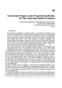
Scheduling Model

Tasks are assigned in order of their dependence. The parallel processors are considered to be fully interconnected. Each task has its processing time ( weight of the task). Tasks communicating across processors incur a communication cost (weight of the edge).

February 2014

OptALI014

Problem and Motivation Scheduling Our Contribution Experimental Results Summary

Scheduling Model Constraints Bi-linear Forms

Outline 1

2

3

Problem and Motivation Scheduling Scheduling Model Constraints Bi-linear Forms Our Contribution Speeding up the Formulation Discussion of Proposed MILP Formulation

4

Experimental Results

5

Summary February 2014

OptALI014

Problem and Motivation Scheduling Our Contribution Experimental Results Summary

Scheduling Model Constraints Bi-linear Forms

Constraints(Tasks on Same processor)

Given by task graph

G = (V , E )

Li : execution time of task i weight of node

p p p p

Processor constraint ( i = j )  i= j⇒ February 2014

or

ti + Li ≤ tj tj + Lj ≤ ti OptALI014

Problem and Motivation Scheduling Our Contribution Experimental Results Summary

Scheduling Model Constraints Bi-linear Forms

Constraints(Tasks on Same processor)

Given by task graph

G = (V , E )

Li : execution time of task i weight of node

p p p p

Processor constraint ( i = j )  i= j⇒ February 2014

or

ti + Li ≤ tj tj + Lj ≤ ti OptALI014

Problem and Motivation Scheduling Our Contribution Experimental Results Summary

Scheduling Model Constraints Bi-linear Forms

Constraints(Tasks on Same processor)

Given by task graph

G = (V , E )

Li : execution time of task i weight of node

p p p p

Processor constraint ( i = j )  i= j⇒ February 2014

or

ti + Li ≤ tj tj + Lj ≤ ti OptALI014

Problem and Motivation Scheduling Our Contribution Experimental Results Summary

Scheduling Model Constraints Bi-linear Forms

Constraints(Tasks on dierent processor)

p p  pi 6= pj ⇒ or ttij ≤≤ ttji

Processor constraint ( i 6= j )

p p i j tj ≥ ti + Li + γij

Processor constraint ( i 6= j and edge → )

i

γij : remote communication cost between tasks and weight of edgeFebruary 2014

OptALI014

j

Problem and Motivation Scheduling Our Contribution Experimental Results Summary

Scheduling Model Constraints Bi-linear Forms

Constraints(Tasks on dierent processor)

p p  pi 6= pj ⇒ or ttij ≤≤ ttji

Processor constraint ( i 6= j )

p p i j tj ≥ ti + Li + γij

Processor constraint ( i 6= j and edge → )

i

γij : remote communication cost between tasks and weight of edgeFebruary 2014

OptALI014

j

Problem and Motivation Scheduling Our Contribution Experimental Results Summary

Scheduling Model Constraints Bi-linear Forms

Outline 1

2

3

Problem and Motivation Scheduling Scheduling Model Constraints Bi-linear Forms Our Contribution Speeding up the Formulation Discussion of Proposed MILP Formulation

4

Experimental Results

5

Summary February 2014

OptALI014

Problem and Motivation Scheduling Our Contribution Experimental Results Summary

Scheduling Model Constraints Bi-linear Forms

Bi-linear Forms

Communication costs arises between tasks with an edge running on dierent processors They give rise to bilinear forms that needs to be linearised February 2014

OptALI014

Problem and Motivation Scheduling Our Contribution Experimental Results Summary

Scheduling Model Constraints Bi-linear Forms

Bi-linear Forms

How do they look like?

February 2014

OptALI014

Problem and Motivation Scheduling Our Contribution Experimental Results Summary

Scheduling Model Constraints Bi-linear Forms

Bi-linear Forms

i

h

( 1 task runs on processsor , ih = 0 otherwise.

x Let Let Let Let

ti be the start time of task i . tj be the start time of task j . Li be the execution time of task i .

i

j

γij be the communication cost between tasks and .

Constraints for remote communication is bi-linear

j V : i ∈ δ − (j )

∀ ∈

ti + Li +

February 2014

x x

t

∑ γij ( ih . jk ) ≤ j h,k ∈P

OptALI014

Problem and Motivation Scheduling Our Contribution Experimental Results Summary

Scheduling Model Constraints Bi-linear Forms

Bi-linear Forms

j V : i ∈ δ −(j )

∀ ∈

ti + Li +

x x

t

∑ γij ( ih . jk ) ≤ j h,k ∈P

where

j V : i ∈ δ −(j ), h, k ∈ P (z hkij = xih .xjk ).

∀ ∈

x x

The boolean multiplication of ih . jk needs to be linearised How is the linearisation done?

February 2014

OptALI014

Problem and Motivation Scheduling Our Contribution Experimental Results Summary

Scheduling Model Constraints Bi-linear Forms

Bi-linear Forms

j V : i ∈ δ −(j )

∀ ∈

ti + Li +

x x

t

∑ γij ( ih . jk ) ≤ j h,k ∈P

where

j V : i ∈ δ −(j ), h, k ∈ P (z hkij = xih .xjk ).

∀ ∈

x x

The boolean multiplication of ih . jk needs to be linearised How is the linearisation done?

February 2014

OptALI014

Problem and Motivation Scheduling Our Contribution Experimental Results Summary

Scheduling Model Constraints Bi-linear Forms

Bi-linear Forms

j V : i ∈ δ −(j )

∀ ∈

ti + Li +

x x

t

∑ γij ( ih . jk ) ≤ j h,k ∈P

where

j V : i ∈ δ −(j ), h, k ∈ P (z hkij = xih .xjk ).

∀ ∈

x x

The boolean multiplication of ih . jk needs to be linearised How is the linearisation done?

February 2014

OptALI014

Problem and Motivation Scheduling Our Contribution Experimental Results Summary

Scheduling Model Constraints Bi-linear Forms

Bi-linear Forms Method 1: The usual approach

j V : i ∈ δ −(j )

∀ ∈

ti + Li +

j V , i ∈ δ −(j ), h, k ∈ P j V , i ∈ δ −(j ), h, k ∈ P j V , i ∈ δ −(j ), h, k ∈ P

∀ ∈ ∀ ∈ ∀ ∈

February 2014

x x

t

∑ γij ( ih . jk ) ≤ j h,k ∈P

xih ≥ z hkij xjk ≥ z hkij xih + xjk − 1 ≤ z hkij

OptALI014

(0)

(1) (2) (3)

Problem and Motivation Scheduling Our Contribution Experimental Results Summary

Scheduling Model Constraints Bi-linear Forms

Bi-linear Forms Method 1: The usual approach

j V : i ∈ δ −(j )

∀ ∈

ti + Li +

j V , i ∈ δ −(j ), h, k ∈ P j V , i ∈ δ −(j ), h, k ∈ P j V , i ∈ δ −(j ), h, k ∈ P

∀ ∈ ∀ ∈ ∀ ∈

February 2014

x x

t

∑ γij ( ih . jk ) ≤ j h,k ∈P

xih ≥ z hkij xjk ≥ z hkij xih + xjk − 1 ≤ z hkij

OptALI014

(0)

(1) (2) (3)

Problem and Motivation Scheduling Our Contribution Experimental Results Summary

Scheduling Model Constraints Bi-linear Forms

Bi-linear Forms

j V : i ∈ δ −(j )

∀ ∈

ti + Li +

x x

t

∑ γij ( ih . jk ) ≤ j h,k ∈P

(0)

Method 2: The compact linearisation

i j V ,k ∈ P ∀i 6= j ∈ V , h, k ∈ P ∀ 6= ∈

z

x

∑ hk ij = jk h∈P hk = kh ij ji

z

February 2014

z

OptALI014

(4) (5)

Problem and Motivation Scheduling Our Contribution Experimental Results Summary

Scheduling Model Constraints Bi-linear Forms

Bi-linear Forms

j V : i ∈ δ −(j )

∀ ∈

ti + Li +

x x

t

∑ γij ( ih . jk ) ≤ j h,k ∈P

(0)

Method 2: The compact linearisation

i j V ,k ∈ P ∀i 6= j ∈ V , h, k ∈ P ∀ 6= ∈

z

x

∑ hk ij = jk h∈P hk = kh ij ji

z

February 2014

z

OptALI014

(4) (5)

Problem and Motivation Scheduling Our Contribution Experimental Results Summary

Scheduling Model Constraints Bi-linear Forms

Bi-linear Forms (Eq. 4) is obtained by multiplying both sides of the equality (Eq. 6) with

x

i j V , k ∈ P.

with jk ; ∀ 6= ∈

i V

x

(6) ∑ ih = 1 h∈P Eq 6. implies that any given task can run on exactly one processor. ∀ ∈

Method 2: The compact linearisation

i j V ,k ∈ P ∀i 6= j ∈ V , h, k ∈ P ∀ 6= ∈

z

x

∑ hk ij = jk h∈P hk = kh ij ji

z

February 2014

z

OptALI014

(4) (5)

Problem and Motivation Scheduling Our Contribution Experimental Results Summary

Scheduling Model Constraints Bi-linear Forms

Bi-linear Forms Problems?

z Result in a high number of variables, O (|V | |P | ) . Linearisation step uses an additional variable . 2

2

First linearisation method has a constraint complexity of (| || 2 |).

O E P

Second linearisation method has a constraint complexity of (| 2 || |).

O V P

Can we get rid of it?

Yes, we use problem specic knowledge Why get rid of it?

Eliminate

z variable and the associated constraint complexity. February 2014

OptALI014

Problem and Motivation Scheduling Our Contribution Experimental Results Summary

Scheduling Model Constraints Bi-linear Forms

Bi-linear Forms Problems?

z Result in a high number of variables, O (|V | |P | ) . Linearisation step uses an additional variable . 2

2

First linearisation method has a constraint complexity of (| || 2 |).

O E P

Second linearisation method has a constraint complexity of (| 2 || |).

O V P

Can we get rid of it?

Yes, we use problem specic knowledge Why get rid of it?

Eliminate

z variable and the associated constraint complexity. February 2014

OptALI014

Problem and Motivation Scheduling Our Contribution Experimental Results Summary

Scheduling Model Constraints Bi-linear Forms

Bi-linear Forms Problems?

z Result in a high number of variables, O (|V | |P | ) . Linearisation step uses an additional variable . 2

2

First linearisation method has a constraint complexity of (| || 2 |).

O E P

Second linearisation method has a constraint complexity of (| 2 || |).

O V P

Can we get rid of it?

Yes, we use problem specic knowledge Why get rid of it?

Eliminate

z variable and the associated constraint complexity. February 2014

OptALI014

Problem and Motivation Scheduling Our Contribution Experimental Results Summary

Scheduling Model Constraints Bi-linear Forms

Bi-linear Forms Problems?

z Result in a high number of variables, O (|V | |P | ) . Linearisation step uses an additional variable . 2

2

First linearisation method has a constraint complexity of (| || 2 |).

O E P

Second linearisation method has a constraint complexity of (| 2 || |).

O V P

Can we get rid of it?

Yes, we use problem specic knowledge Why get rid of it?

Eliminate

z variable and the associated constraint complexity. February 2014

OptALI014

Problem and Motivation Scheduling Our Contribution Experimental Results Summary

Scheduling Model Constraints Bi-linear Forms

Bi-linear Forms Problems?

z Result in a high number of variables, O (|V | |P | ) . Linearisation step uses an additional variable . 2

2

First linearisation method has a constraint complexity of (| || 2 |).

O E P

Second linearisation method has a constraint complexity of (| 2 || |).

O V P

Can we get rid of it?

Yes, we use problem specic knowledge Why get rid of it?

Eliminate

z variable and the associated constraint complexity. February 2014

OptALI014

Problem and Motivation Scheduling Our Contribution Experimental Results Summary

Speeding up the Formulation Discussion of Proposed MILP Formulation

Outline 1

2

3

Problem and Motivation Scheduling Scheduling Model Constraints Bi-linear Forms Our Contribution Speeding up the Formulation Discussion of Proposed MILP Formulation

4

Experimental Results

5

Summary February 2014

OptALI014

Problem and Motivation Scheduling Our Contribution Experimental Results Summary

Speeding up the Formulation Discussion of Proposed MILP Formulation

First Contribution

Formulate a simple and eective linearisation for the Bi-Linear forms arising out of communication delays. All linearisation variables | |2 | |2 , variables.

V P z

z are eliminated freeing upto

February 2014

OptALI014

Problem and Motivation Scheduling Our Contribution Experimental Results Summary

Speeding up the Formulation Discussion of Proposed MILP Formulation

Outline 1

2

3

Problem and Motivation Scheduling Scheduling Model Constraints Bi-linear Forms Our Contribution Speeding up the Formulation Discussion of Proposed MILP Formulation

4

Experimental Results

5

Summary February 2014

OptALI014

Problem and Motivation Scheduling Our Contribution Experimental Results Summary

Speeding up the Formulation Discussion of Proposed MILP Formulation

Proposed MILP Formulation: Overlap Variables

Overlap Variables

ij V

σij

ij V

εij

∀, ∈

∀, ∈

( 1 = 0 ( 1 = 0

i

j

task nishes before task starts otherwise

i

the PI∗ of task is strictly less than task otherwise

* PI is the Processor Index

February 2014

OptALI014

j

Problem and Motivation Scheduling Our Contribution Experimental Results Summary

Speeding up the Formulation Discussion of Proposed MILP Formulation

Proposed MILP Formulation: Overlap Variables

Overlap Variables

ij V

σij

ij V

εij

∀, ∈

∀, ∈

( 1 = 0 ( 1 = 0

i

j

task nishes before task starts otherwise

i

the PI∗ of task is strictly less than task otherwise

* PI is the Processor Index

February 2014

OptALI014

j

Problem and Motivation Scheduling Our Contribution Experimental Results Summary

Speeding up the Formulation Discussion of Proposed MILP Formulation

Proposed ILP Formulation Constraints

min W i V ti + Li ≤ W i j V εij + εji ≤ 1 i j V σij + σji ≤ 1 i j V σij + σji + εij + εji ≥ 1 j V i j σij = 1 i j V pj − pi − 1 − (εij − 1)|P | ≥ 0 i j V tj − ti − Li − (σij − 1)Wmax ≥ 0 j V i j h k P ti + Li + γ hkij (xih + xjk − 1) ≤ tj j V i j ti + Li ≤ tj i V ∑ xik = 1 kεP ∀i ∈ V ∑ kxik = pi

∀ ∈ ∀ 6= ∈ ∀ 6= ∈ ∀ 6= ∈ ∀ ∈ : ∈ δ −( ) ∀ 6= ∈ ∀ 6= ∈ ∀ ∈ : ∈ δ − ( ), ∀ , ∈ ∀ ∈ : ∈ δ −( ) ∀ ∈

kεP

February 2014

OptALI014

MinM

Overla

Edge

Proces

Time

Connect

Problem and Motivation Scheduling Our Contribution Experimental Results Summary

Speeding up the Formulation Discussion of Proposed MILP Formulation

Formulation Bounds

W ≥0 ti ≥ 0

i ∈V i ∈ V pi ∈ {1, . . . , |P |} i V , k ∈ P xik ∈ {0, 1} i j ∈ V σij , εij ∈ {0, 1}

∀ ∀ ∀ ∈ ∀,

February 2014

OptALI014

Problem and Motivation Scheduling Our Contribution Experimental Results Summary

Speeding up the Formulation Discussion of Proposed MILP Formulation

Proposed ILP Formulation ( 1 ih = 0 ( 1 jk = 0

x x

task

i

runs on processsor ,

h

j

runs on processsor ,

otherwise. task

k

otherwise.

j V : i ∈ δ −(j ), ∀h, k ∈ P ∀j ∈ V : i ∈ δ − (j )

∀ ∈

ti + Li + γ hkij (xih + xjk − 1) ≤ tj ti + Li ≤ tj

Done only for tasks with edges Also equivalent to a Boolean multiplication.

x

x

The second equation compensates when ih and jk are both 0 February 2014

OptALI014

Problem and Motivation Scheduling Our Contribution Experimental Results Summary

Speeding up the Formulation Discussion of Proposed MILP Formulation

Proposed ILP Formulation ( 1 ih = 0 ( 1 jk = 0

x x

task

i

runs on processsor ,

h

j

runs on processsor ,

otherwise. task

k

otherwise.

j V : i ∈ δ −(j ), ∀h, k ∈ P ∀j ∈ V : i ∈ δ − (j )

∀ ∈

ti + Li + γ hkij (xih + xjk − 1) ≤ tj ti + Li ≤ tj

Done only for tasks with edges Also equivalent to a Boolean multiplication.

x

x

The second equation compensates when ih and jk are both 0 February 2014

OptALI014

Problem and Motivation Scheduling Our Contribution Experimental Results Summary

Speeding up the Formulation Discussion of Proposed MILP Formulation

Proposed ILP Formulation ( 1 ih = 0 ( 1 jk = 0

x x

task

i

runs on processsor ,

h

j

runs on processsor ,

otherwise. task

k

otherwise.

j V : i ∈ δ −(j ), ∀h, k ∈ P ∀j ∈ V : i ∈ δ − (j )

∀ ∈

ti + Li + γ hkij (xih + xjk − 1) ≤ tj ti + Li ≤ tj

Done only for tasks with edges Also equivalent to a Boolean multiplication.

x

x

The second equation compensates when ih and jk are both 0 February 2014

OptALI014

Problem and Motivation Scheduling Our Contribution Experimental Results Summary

Speeding up the Formulation Discussion of Proposed MILP Formulation

Proposed ILP Complexity

Bi-Linear 1

VARIABLES

E P z

| |.| | , variables 2

February 2014

Bi-Linear 2

Improved-1[3

| | .| | , variables

free of

V P z 2

OptALI014

2

z

Problem and Motivation Scheduling Our Contribution Experimental Results Summary

Speeding up the Formulation Discussion of Proposed MILP Formulation

Proposed ILP

min W ∀i ∈ V ti + Li ≤ W ∀i 6= j ∈ V εij + εji ≤ 1 ∀i 6= j ∈ V σij + σji ≤ 1 ∀i 6= j ∈ V σij + σji + εij + εji ≥ 1 ∀j ∈ V : i ∈ δ − (j ) σij = 1 ∀i 6= j ∈ V pj − pi − 1 − (εij − 1)|P | ≥ 0 ∀i 6= j ∈ V tj − ti − Li − (σij − 1)Wmax ≥ 0 ∀j ∈ V : i ∈ δ − (j ), ∀h, k ∈ P ti + Li + γ hk ij (xih + xjk − 1) ≤ tj − ∀j ∈ V : i ∈ δ (j ) ti + Li ≤ tj ∀i ∈ V ∑ xik = 1 kεP ∀i ∈ V ∑ kxik = pi kεP

February 2014

OptALI014

Problem and Motivation Scheduling Our Contribution Experimental Results Summary

Speeding up the Formulation Discussion of Proposed MILP Formulation

Improve Proposed ILP

If we are able to remove all processor indices running on the subscript, the constraint complexity reduces from (| |2 +| || |2 ) to (| |2 )

O V

E P

O V

We however retain the bounds on the processors for the number of processors to be nitely bounded

i V

∀ ∈

pi ∈ {1, . . ., |P |}

February 2014

OptALI014

Problem and Motivation Scheduling Our Contribution Experimental Results Summary

Speeding up the Formulation Discussion of Proposed MILP Formulation

Improve Proposed ILP

If we are able to remove all processor indices running on the subscript, the constraint complexity reduces from (| |2 +| || |2 ) to (| |2 )

O V

E P

O V

We however retain the bounds on the processors for the number of processors to be nitely bounded

i V

∀ ∈

pi ∈ {1, . . ., |P |}

February 2014

OptALI014

Problem and Motivation Scheduling Our Contribution Experimental Results Summary

Speeding up the Formulation Discussion of Proposed MILP Formulation

Improved Proposed ILP

min ∀i ∈ V ∀i 6= j ∈ V ∀i 6= j ∈ V ∀i 6= j ∈ V ∀i 6= j ∈ V ∀i 6= j ∈ V ∀i 6= j ∈ V ∀j ∈ V : i ∈ δ − (j ) ∀j ∈ V : i ∈ δ − (j )

W ti + Li ≤ W

(1) (2)

σij + σji ≤ 1 (3) εij + εji ≤ 1 (4) σij + σji + εij + εji ≥ 1 (5) j − i − 1 − (εij − 1)| | ≥ 0 (6) j − i − εij | | ≤ 0 (7)

p p

p p

P P

ti + Li + (σij − 1)Wmax ≤ tj ti + Li + γij (εij + εji ) ≤ tj

(8) (9)

σij = 1 (10)

February 2014

OptALI014

Problem and Motivation Scheduling Our Contribution Experimental Results Summary

Speeding up the Formulation Discussion of Proposed MILP Formulation

Improved ILP Bounds

ij V ∀i ∈ V ∀i ∈ V

σij , εij ∈ {0, 1} (11) i ∈ {1, . . ., | |} (12)

∀, ∈

p ∑ Li + ∑

i ∈V

February 2014

i ,j ∈V

OptALI014

γij −

P

ti ≥ 0 W ≥0

Wmax = 0

(13) (14) (15)

Problem and Motivation Scheduling Our Contribution Experimental Results Summary

Speeding up the Formulation Discussion of Proposed MILP Formulation

Improve Proposed ILP

j V : i ∈ δ −(j ),∀h, k ∈ P ti + Li + γ hkij (xih + xjk − 1) ≤ tj ∀j ∈ V : i ∈ δ − (j ) ti + Li ≤ tj ∀i ∈ V ∑ xik = 1 kεP ∀i ∈ V ∑ kxik = pi kεP ∀i ∈ V , k ∈ P xik ∈ {0, 1}

∀ ∈

Are the constarints that left the ILP

February 2014

OptALI014

Problem and Motivation Scheduling Our Contribution Experimental Results Summary

Speeding up the Formulation Discussion of Proposed MILP Formulation

Improve Proposed ILP

Two more very problem specic improvmenets were done NOT discussed but the main ideas have been presented

February 2014

OptALI014

Problem and Motivation Scheduling Our Contribution Experimental Results Summary

Experimental Results The computations are carried out using CPLEX 11.0 on an Intel Core i3 processor 330M, 2.13 GHZ CPU and 2 GB RAM running with no parallel mode and on a single thread on Windows 7. Graph

n p 20

BI-LINEAR

PROPOSED-1

PROPOSED-2

12h 32.09%

12h 26.15%

12h 25.78%

8

35m:56s

6m:11s

6s

16

12h 3.92%

1h:38m:5s

10s

2 4

ogra20_55

8m:49s

February 2014

18s

OptALI014

14s

Problem and Motivation Scheduling Our Contribution Experimental Results Summary

Experimental Results The computations are carried out using CPLEX 11.0 on an Intel Core i3 processor 330M, 2.13 GHZ CPU and 2 GB RAM running with no parallel mode and on a single thread on Windows 7. Graph

n p 20

BI-LINEAR

PROPOSED-1

PROPOSED-2

12h 32.09%

12h 26.15%

12h 25.78%

8

35m:56s

6m:11s

6s

16

12h 3.92%

1h:38m:5s

10s

2 4

ogra20_55

8m:49s

February 2014

18s

OptALI014

14s

Problem and Motivation Scheduling Our Contribution Experimental Results Summary

Experimental Results The computations are carried out using CPLEX 11.0 on an Intel Core i3 processor 330M, 2.13 GHZ CPU and 2 GB RAM running with no parallel mode and on a single thread on Windows 7. Graph

n p 20

BI-LINEAR

PROPOSED-1

PROPOSED-2

12h 32.09%

12h 26.15%

12h 25.78%

8

35m:56s

6m:11s

6s

16

12h 3.92%

1h:38m:5s

10s

2 4

ogra20_55

8m:49s

February 2014

18s

OptALI014

14s

Problem and Motivation Scheduling Our Contribution Experimental Results Summary

Experimental Results Graph

n p 30

t30_56_1

BI-LINEAR

PROPOSED-1

PROPOSED-2

2

9s

2s

16s

4

7m:32s

17s

32s

8

7h:22m:19s

16

12h 8.94%

12h 0.21% 12h 4.07%

h: Hours m:minutes s:seconds February 2014

OptALI014

48s 15s

Problem and Motivation Scheduling Our Contribution Experimental Results Summary

Experimental Results Graph

n p 30

t30_56_1

BI-LINEAR

PROPOSED-1

PROPOSED-2

2

9s

2s

16s

4

7m:32s

17s

32s

8

7h:22m:19s

16

12h 8.94%

12h 0.21% 12h 4.07%

h: Hours m:minutes s:seconds February 2014

OptALI014

48s 15s

Problem and Motivation Scheduling Our Contribution Experimental Results Summary

Experimental Results Graph

n p 40

2 4

t40_30_1

8 16

BI-LINEAR

PROPOSED-1

PROPOSED-2

6m

46s

3m:29s

29m:33s

4m:25s

12h 7.18% 12h 9.83% 12h 23.66%

12h 5.07% 12h 9.43%

h: Hours m:minutes s:seconds February 2014

OptALI014

3m:34s 4m:3s

Problem and Motivation Scheduling Our Contribution Experimental Results Summary

Experimental Results Graph

n p 40

2 4

t40_30_1

8 16

BI-LINEAR

PROPOSED-1

PROPOSED-2

6m

46s

3m:29s

29m:33s

4m:25s

12h 7.18% 12h 9.83% 12h 23.66%

12h 5.07% 12h 9.43%

h: Hours m:minutes s:seconds February 2014

OptALI014

3m:34s 4m:3s

Problem and Motivation Scheduling Our Contribution Experimental Results Summary

Experimental Results Graph

n p 50

2 4

Ogra50_53

8 16

BI-LINEAR

PROPOSED-1

PROPOSED-2

12h 46.33% 12h 19.78% 12h inf 12h inf

12h 46.15% 12h 5.26%

12h 48.50% 12h 12.94%

February 2014

12h 2.46% 12h 5.58%

OptALI014

17m:17s 58m:2s

Problem and Motivation Scheduling Our Contribution Experimental Results Summary

Summary A MILP formulation to solve the Multi-Processor Scheduling with Communication Delays was proposed[1]. The proposed formulation is free of linearisation variables required to linearise bi-linear forms arising out of comunication delays[2]. All variable subscripts are independent of the number of processors.

V

As a result the constraint complexity reduces to O(| |)2 .

February 2014

OptALI014

Problem and Motivation Scheduling Our Contribution Experimental Results Summary

Summary A MILP formulation to solve the Multi-Processor Scheduling with Communication Delays was proposed[1]. The proposed formulation is free of linearisation variables required to linearise bi-linear forms arising out of comunication delays[2]. All variable subscripts are independent of the number of processors.

V

As a result the constraint complexity reduces to O(| |)2 .

February 2014

OptALI014

Problem and Motivation Scheduling Our Contribution Experimental Results Summary

Summary A MILP formulation to solve the Multi-Processor Scheduling with Communication Delays was proposed[1]. The proposed formulation is free of linearisation variables required to linearise bi-linear forms arising out of comunication delays[2]. All variable subscripts are independent of the number of processors.

V

As a result the constraint complexity reduces to O(| |)2 .

February 2014

OptALI014

Problem and Motivation Scheduling Our Contribution Experimental Results Summary

Summary A MILP formulation to solve the Multi-Processor Scheduling with Communication Delays was proposed[1]. The proposed formulation is free of linearisation variables required to linearise bi-linear forms arising out of comunication delays[2]. All variable subscripts are independent of the number of processors.

V

As a result the constraint complexity reduces to O(| |)2 .

February 2014

OptALI014

Problem and Motivation Scheduling Our Contribution Experimental Results Summary

References

Sarad Venugopalan and Oliver Sinnen, ILP formulations for Optimal Task Scheduling with Communication Delays on Parallel Systems, IEEE Transactions on Parallel and Distributed Systems.DOI: 10.1109/TPDS.2014.2308175, 2014. T. Davidovi¢, L. Liberti, N. Maculan, and N. Mladenovic. Towards the optimal solution of the multiprocessor scheduling problem with communication delays. In , pages 128135, 2007.

3rd Multidisciplinary International Conference on Scheduling: Theory and Application

Sarad Venugopalan and Oliver Sinnen. Optimal linear programming solutions for multiprocessor scheduling with communication delays. In , pages 129138, 2012.

ICA3PP (1)

February 2014

OptALI014