Integrated Backup Topology Control and Routing of. Obscured Traffic in Hybrid RF/FSO Networks*. Abhishek Kashyap, Anuj Rawat and Mark Shayman.
Integrated Backup Topology Control and Routing of Obscured Traffic in Hybrid RF/FSO Networks* Abhishek Kashyap, Anuj Rawat and Mark Shayman Department of Electrical and Computer Engineering, University of Maryland, College Park MD 20742 Email: {kashyap, anuj, shayman}@glue.umd.edu
Abstract— We propose a framework for providing instantaneous backup to traffic in a hybrid RF/FSO mesh network. Free Space Optical (FSO) links have high bandwidth and security, making them suitable for use in backbone networks. RF links have low bandwidth, but offer high reliability in conditions where FSO links are obscured. Thus, RF links are primarily used to provide instantaneous backup to traffic flowing on FSO links. We propose a framework to model FSO link failures due to obscuration, and propose algorithms for integrated topology control of RF links and routing for maximizing the backup provided. We do extensive simulations to demonstrate that the performance of RF topology and routing computed using our algorithms is much better than the case of having the same RF and FSO topologies and routes.
I. I NTRODUCTION Free Space Optical (FSO) links are an alternative to optical fibers for deployment in wireless mesh networks due to their attractive characteristics [1], [2]. FSO links are very easy to deploy and have high capacity and ultra-low interference; these properties make them suitable for backbones in military applications and also for the backbones in wireless mesh networks [3]. One major drawback of FSO links is the high attenuation in fog and snow, which disrupts the traffic flowing through the affected links. RF links are more reliable than FSO links, and can be deployed as easily as FSO links. But, they are not as suitable for mesh networks as the FSO links due to their low capacity, high interference and low security. Since fiber is too expensive and time-consuming to deploy, and both FSO and RF links have drawbacks, hybrid RF/FSO networks have been gaining attention as they lead to a reliable, high-capacity and easy to deploy backbone. The FSO links are used to carry the network traffic, and the RF links are used to provide backup to the network traffic. An RF link typically has a much lower capacity (1:20) compared to an FSO link. Thus, they are primarily used to provide instantaneous backup to a fraction of the traffic. Rerouting on FSO topology can be done for the remaining failed traffic, but that incurs a certain delay. Kashyap et al. [4] proposed a framework to characterize the traffic by its criticality in terms of the real-time flows between each ingress-egress pair. Then, a routing scheme was proposed to maximize the throughput on the FSO topology and maximize the minimum criticality-weighted backup provided to the traffic on the RF topology. The work assumed that the *This research was partially supported by AFOSR under grant F496200210217 and NSF under grant CNS-0435206.
transmitters and receivers at each node have the same aperture for RF and FSO links, i.e., the RF and FSO topologies are identical. In this paper we consider the case where RF and FSO links have different apertures, and thus the two topologies can be different. We propose algorithms for finding an RF topology and backup routing for a given FSO topology and routing. We assume each node has a limited transmission range, and define a neighbor to be a node within the transmission range of another. The nodes are assumed to have a constraint on the number of transmitters and receivers (interfaces), and thus a node cannot form a link with all its neighbors. Since the problem of finding a connected topology with these interface constraints is NP-Hard [5], the corresponding problem of integrated routing and topology control is NP-Hard as well [6]. We model the failures due to obscuration as the failure of regions in an overlapping partition of the network area. Failure of a region (which we call a grid) leads to the obscuration of all FSO links originating, ending or passing through the grid. We assign probabilities of failure to the individual grids, and use path decomposition to compute the traffic that would be affected if a grid is obscured. One option would be to have an RF topology and routing corresponding to each grid failure, and set it up when a grid fails. The topology and routing can be computed using the integrated topology control and routing algorithms of [6], [7], [8]. However, this would incur a delay in providing the backup, which defeats the purpose of having RF links in the network. RF links are included in the network in order to provide instantaneous backup to the affected traffic, and thus the backup traffic should be flowing on the RF network when a failure occurs. Thus, we compute a single RF topology and routing, that performs well for any grid failure. There has been a considerable amount of work in wireline optical networks for backup topology control of lightpaths and routing, but all of them assume single link or node failures and provide link or node disjoint paths for protection of each path (see [9] for an ILP formulation of the problem). One may want to view RF links as an additional wavelength in wireline networks, to be used only for backup, and try to apply the same algorithms. However, there is a very important difference between the two problems: single link (node) failure assumption is not valid for wireless optical networks where failures are usually due to weather conditions that affect a whole region (leading to the failure of all links in that region). Thus, the algorithms proposed for wireline optical networks cannot be used for hybrid RF/FSO networks.
We compare our algorithms with a currently employed backup technique [10], in which the RF topology is the same as the FSO topology and the RF backup routes are the same as the corresponding routes on the FSO topology. We show via extensive simulations that the proposed algorithms lead to an improvement in the backup provided. The improvement is as high as 50% if the FSO topology is not optimized for the current network traffic. We note that this would actually be the case since modification of FSO topology leads to disruption of flows on the network, and thus the FSO topology is not modified too often, so it may not be optimized for the current traffic. However, the RF topology can be modified at any time since it carries backup flows. Also, since the FSO links usually have ample bandwidth, it is not desirable to modify the FSO topology as traffic profile changes. However, RF links have very low bandwidth and thus need to be reconfigured frequently. To the best of our knowledge, this is the first framework of modelling failures and providing backup to traffic in hybrid RF/FSO networks, along with the algorithms for integrated RF topology control and routing to achieve the proposed backup objectives. The idea of having a criticality index associated with each ingress-egress pair [4] can be easily incorporated in our framework and algorithms. The paper is organized as follows: Section 2 gives the network model and problem definition, along with failure modelling. Section 3 presents the algorithms we propose for integrated RF topology control and routing. Section 4 gives the computational complexity and simulation results, and Section 5 concludes the paper. II. N ETWORK M ODEL AND P ROBLEM D EFINITION We consider a hybrid RF/FSO backbone network where each node is capable of routing. We assume that the transmitters and receivers at each node have a different aperture for RF and FSO links. Thus, the RF and FSO topologies can be different. We also assume that the network nodes have a fixed number of transmitters and receivers, and a limited transmission range. We assume the RF and FSO links are unidirectional. We assume both the RF and FSO transmission range as well as the number of RF and FSO interfaces (transmitters and receivers) available per node to be the same. Due to the interface and transmission range constraints, a node ni can connect to another node nj via an RF (FSO) link only if nj lies in ni ’s RF (FSO) transmission range and there is a free RF (FSO) transmitter and a free RF (FSO) receiver at ni and nj respectively. The capacity of each link is assumed to be fixed depending on the type of the link. The capacity of FSO links is much greater (20:1) than the capacity of RF links. The FSO topology carries all the traffic in the network. Since the FSO links are susceptible to environmental phenomenon such as fog, snow, clouds, etc. (we do not take the effects of scintillation into account), the RF topology is used to provide the necessary backup. In this paper we assume that the FSO topology and the aggregate traffic profile currently being routed, along with the actual routing being used, is given. The
A B
C
D
Fig. 1. Partition of network into grids, each corresponding to a failure event
problem of interest is to determine an RF topology and routing that maximizes the amount of backup provided (as measured according to an appropriate objective function). We now explain the set-up used for modelling failures in the network and the construction of the objective function. Let TF denote the FSO topology, P be the aggregate traffic profile, and RF,P be the routing for this aggregate traffic. The aggregate traffic profile P consists of source-destination (SD) pairs, along with the total traffic being routed between each pair through multiple multi-hop paths. Note that the routing RF,P can be decomposed into paths using flow decomposition [11] to give a set of paths and corresponding flows for each SD pair. Our goal is to provide backup for every individual path corresponding to each SD pair. Thus, we consider each of these paths as a demand. We model the failures in the network as obscuration of certain geographical regions (due to fog/snow/clouds). We partition the overall geographical region spanned by the network into grids of equal area (see Figure 1). Let the region spanned by the network be a square of side L, and each grid be a square of side l. Note that the shape and size of the grids and the region spanned by the network do not matter in our proposed approach: we use square, equal-area grids and square geographical region just for clarity. For our presentation, we consider four overlapping grid structures of Types A, B, C and D, each shifted with respect to the other by l/2 in the directions parallel to the sides of the square grid. Figure 1 depicts the network nodes, the FSO topology, the full grid structure for Type A grids, and a grid for the other grids types. Thus, the total number of grids in the network is G = 4�L/l�2 . We assume that at a time only one grid can fail. Here, by failure of a grid, we mean the failure of all FSO links passing through, originating or ending in that grid. Thus, the traffic originating, ending or passing through that grid can no longer be routed on the FSO topology. The goal is to use the RF links to provide backup to this traffic. Since RF links should provide instantaneous backup for the disrupted traffic, we cannot set-up the RF topology and backup routing after the grid failure. Thus, we compute the backup RF topology and routing taking the possibility of each grid failure into account.
TABLE I N OTATIONS Symbol TF TRF P RF,P RRF,P N G pi Pi tf bf ri cl xlf sf , df On , In
Equation 2b ensures that for every demand in Pi , a minimum fraction ri of the disrupted traffic is backed up. Thus, ri measures the minimum fraction of the traffic backed up for all paths (demands) affected when grid i fails. Equations 2d, 2e and 2c represent the flow conservation constraints at the source, the destination and the other network nodes respectively, for every commodity. Equation 2f represents the capacity constraints of RF links, and Equation 2g gives the bounds on the variables.
Definition FSO topology RF topology Aggregate traffic profile Routes on FSO topology Routes on RF topology Number of nodes in the network Number of grids Probability of failure of grid i Set of paths and traffic in RF,P routed through grid i Traffic on path f in RF,P Backup traffic routed on RF topology for path f Minimum fraction backed up among paths in Pi Capacity of RF link l Demand of path f routed on link l in RRF,P or RF,P Source and destination nodes for path f Set of outgoing and incoming edges at node n
G �
pi ri
(2a)
s.t. bf ≥ ri tf , ∀f ∈ Pi , i ∈ {1, ··, G} � � xlf = xlf ,
(2b)
maximize
i=1
l∈Ij
l∈Oj
∀j ∈ {1, .., N } − {sf , df }, ∀f ∈ RF,P We assume that the probability of failure of grid i is pi . Let Pi denote the set of paths (which we call demands) and the corresponding traffic being routed through grid i by routing RF,P (of traffic profile P on FSO topology TF ). We refer to Pi as the traffic profile for grid i. Each profile Pi consists of a subset of demands (paths in RF,P ). The subsets may be overlapping. Since the grids cover the whole network, the union of all profiles Pi contains all the paths in RF,P . We denote the backup routing for aggregate traffic profile P on the RF topology TRF , by RRF,P . We want to determine the RF topology and the backup routing in order to maximize the weighted average of the minimum fraction of backup traffic routed for each grid failure, where the weights correspond to the probability of failure of the individual grids. The objective function is stated in Equation 1. max
TRF ,RRF,P
G � i=1
pi min
f ∈Pi
bf tf
(1)
subject to: TRF satisfies interface and range constraints RRF,P satisfies RF capacity constraints Here the minimum is over the demands in Pi for each grid i, and the weighted average is taken over the grids. Table I provides a list of notations we use in this paper. III. I NTEGRATED T OPOLOGY C ONTROL AND ROUTING In this section, we present algorithms for integrated backup topology control and routing. The procedure for computing routing on a given RF topology is the same in all algorithms, but the algorithms for determining that RF topology differ. We first discuss the procedure for computing a backup routing on a fixed RF topology that maximizes the objective function given in Equation 1. We formulate the problem as a multi-commodity flow problem [12], � where the set of commodities is the set of demands in i Pi , each demand being a commodity. Equation 2 gives a linear program (LP) to solve the routing problem for backup traffic. Equation 2a states the objective.
�
xlf −
l∈Osf
�
�
(2c)
xlf = bf , ∀f ∈ RF,P
(2d)
xlf = bf , ∀f ∈ RF,P
(2e)
l∈Isf
xlf −
l∈Idf
�
�
l∈Odf
xlf ≤ cl , ∀l ∈ TRF
(2f)
f ∈RF,P
ri ≥ 0, 0 ≤ bf ≤ tf , xlf ≥ 0
(2g)
We now present the topology control and routing algorithms. A. Identical Topology and Routing Algorithm (ITRA) Identical Topology and Routing Algorithm (ITRA) assumes the RF topology to be the same as the FSO topology, and restricts the backup RF paths to be identical to the FSO paths. After identifying the RF topology and paths, it solves the LP of Equation 2 to determine the backup for each demand in RF,P in order to maximize the objective value. The restriction of fixing a set of paths can be incorporated in the LP by setting the flow variables xlf to zero for links l which are not in the path for flow f . We will compare our algorithms with ITRA, as it is based on the currently followed algorithms that use the FSO topology and routes for RF [10]. B. Unweighted Matching Based Algorithm (UMBA) Unweighted Matching Based Algorithm (UMBA) proceeds in two stages (steps). In the first step, it constructs a valid RF topology having maximum number of links using maximum weight matching based algorithm proposed in [6]. By valid topology we mean that the topology satisfies the interface and transmission range constraints at every node. Then the algorithm computes the backup routing RRF,P on this RF topology using the LP presented in Equation 2. In the second step, which we call the post-processing step, the algorithm iteratively modifies the RF topology and recomputes the backup routing to improve the value of the objective function. For doing this, a weight wf , as determined by Equation 3, is
Algorithm 1 Post-processing step 1: sort the demands d ∈ RF,P in decreasing order of weights wd (Equation 3) to form criticality list L 2: update ← 0 3: while stopping criteria not reached do 4: pick the next demand f from L 5: if update = 1 then 6: recompute weight wf corresponding to demand f 7: end if 8: if wf = 0 then 9: goto Step 3 10: end if 11: find a set of K shortest paths Π in the potential RF topology between the source sf and the destination df corresponding to demand f 12: if for every path π ∈ Π, every link of π is in the current RF topology TRF then 13: goto Step 3 14: end if 15: add (and delete) the required links in order to form path π in the RF topology 16: determine the routing on the new topology and determine the new objective value nval (let the original objective value be val) 17: if nval > val OR val = 0 then 18: update the RF topology TRF , backup routing RRF,P and the objective value val 19: update ← 1 20: end if 21: end while assigned to every demand f ∈ RF,P . � wf = pi Ibf /tf ≤αri
(3)
i|f ∈Pi
Here, IE is an indicator function that takes value 1 when condition E is true, 0 otherwise. So for any demand f , wf is the probability of failure of critical grids for that demand. Grid i is considered critical with respect to demand f if the failure of grid i disrupts demand f and the fraction of traffic backed up for demand f is less than or equal to a constant (α > 1) times the minimum fraction of traffic backed up for any demand affected by the failure of grid i, i.e., if bf /tf ≤ αri . Clearly a higher value of α leads to higher weights. Moreover, for grids having the minimum fraction of backed up traffic (over demands affected by the failure of that grid) equal to zero, we add a large weight to all the demands affected by the failure of that grid. In other words, if ri = 0 for grid i, we add a large weight (� maxi pi ) to every demand f ∈ Pi . This is done to ensure that we have some (non-zero) backup for all demands disrupted due to any possible grid failure. The algorithm then sorts the list of demands (referred to as the criticality list) in decreasing order of weights, and modifies the RF topology in order to achieve a better objective value. The algorithm picks each entry (demand) from the criticality
list and finds up to K shortest routes (of same length) for the SD pair of that demand in the potential RF topology. By potential topology we mean a topology in which every node is connected to all nodes within its transmission range irrespective of the interface constraints. Then the algorithm finds the first of these K routes that does not exist in the current RF topology, TRF . If such a route exists, the algorithm modifies the current RF topology by forming this route. To form the route, we add the links in the topology which are present in the route, but not in TRF . Due to the interface constraints, it may not be possible to add the new links required without deleting some of the existing links. Suppose we need to add link ni −→ nj to the topology, but all the transmitters at node ni are being used or/and all the receivers at node nj are being used. The algorithm deletes the least loaded link (in routing RRF,P ) from among the outgoing links at the nodes where it needs a transmitter, and deletes the least loaded link from among the incoming links at the nodes where it needs a free receiver. The algorithm then recomputes the routing and the value of the objective function. If the new objective value is greater than the previous objective value, the RF topology TRF and the routing RRF,P are updated, otherwise the changes are discarded and the algorithm keeps the old RF topology and routing. Note that an objective value of zero indicates that the topology is disconnected. Thus, if the old objective value was zero, we change the topology to the new one even if the new objective value is zero as well. We do this to try to make the topology connected. Simulations showed that we could connect all topologies which were disconnected after Step 1. Then, the algorithm picks the next entry from the criticality list and recomputes (if required) the weight for this demand using the updated routing. If the weight is zero and the current objective value is not zero, then the entry is discarded. Otherwise the demand is processed as described before. We stop the iterations in the post-processing step when any of the following two stopping criteria is reached. • •
All the entries of the criticality list have been either processed or discarded. At least ten entries of the criticality list have been processed and the objective value has not changed after the processing of last five entries.
The post-processing step is presented in Algorithm 1. C. Traffic Weighted Matching Based Algorithm (TWMBA) Traffic Weighted Matching Based Algorithm (TWMBA) differs from UMBA in the initial RF topology that it constructs. The algorithm constructs a valid RF topology based on traffic weighted matching [6]. The traffic weighted matching algorithm constructs a topology that attempts to maximize throughput for a given traffic profile. The traffic profile we use for the purpose is the aggregate traffic profile in the FSO network, P. The traffic weighted matching based algorithm was shown to have a better performance than the unweighted matching based algorithm. This is used as the initial RF
topology. The post-processing step and the computation of routing is the same as in UMBA. D. Weighted Profile Weighted Matching Based Algorithm (WPWMBA) Weighted Profile Weighted Matching Based Algorithm (WPWMBA) differs from UMBA in the initial RF topology that it constructs. The algorithm constructs a new traffic profile, P � , that is a weighted sum of the traffic profiles Pi for every grid i ∈ {1, . . . , G}. The probability of failure of grids is used for weighting the corresponding traffic profiles. Equation 4 gives the relation between the new traffic profile P � and the grid traffic profiles. Since Pi s can be overlapping, some paths may be counted multiple times in the constructed profile P � . This is desirable since a path is more likely to fail if it passes through more grids, or through grids with higher failure probability. Thus, the traffic for each path in Pi is proportional to the sum of failure probabilities of the grids it passes through. � P� = pi Pi (4) i∈{1,...,G}
The algorithm then constructs a valid RF topology based on traffic weighted matching using traffic profile P � . This is used as the initial RF topology. The post-processing step and the computation of routing is the same as in UMBA. IV. C OMPUTATIONAL C OMPLEXITY AND S IMULATION R ESULTS A. Computational Complexity Solving a linear program using interior point method takes O(n3.5 ) time [13], where n is the number of constraints in the LP. Hence, we require O((GN 3 +N 4 +E)3.5 ) = O(G3.5 N 14 ) time for solving the LP of Equation 2. Here, G is the number of grids, E is the number of edges in the topology and N is the number of nodes in the network. However, the actual time taken by LP solvers like CPLEX [14] is much less, and the worst case complexity is misleading. We denote the time taken for solving an LP as O(f (N, G)). The step of computing an initial RF topology in UMBA, TWMBA and WPWMBA using maximum weight matching takes O(N 4 logN ) time [6]. The post-processing step has O(N 3 ) iterations, and each iteration requires solving the LP of Equation 2 once. Thus, ITRA takes O(f (N, G)) time; UMBA, TWMBA and WPWMBA take O(N 4 logN + N 3 f (N, G)) time. B. Simulation Results and Discussion The networks simulated were in a square region of side length 3km. The networks had 20 nodes, each having a transmission range of 1km. The node locations were independently chosen uniformly randomly in the network. The number of transmit and receive interfaces at every node was taken to be 4. The traffic for FSO network (constituting the primary traffic profile P) was generated between each node pair in the network, and was uniform random between 20 and 40 Mbps. The RF link capacity was assumed to be 100 Mbps. The FSO links were assumed to have a capacity large enough to support
the primary traffic, and the routing RF,P of primary traffic was assumed to be the one that leads to minimum link load. Equation 5 gives the linear program we use to compute the primary routing on a given FSO topology, which is formulated as a multi-commodity flow problem. The traffic profile P consists of demands f , each requiring traffic tf to be routed, which is treated as a commodity. The maximum link load is represented by σ. The rest of the notations are the same as in Table I. Equation 5a presents the objective function that minimizes the link load σ. The constraints of Equation 5b ensure the load on each link is below σ. Equations 5c, 5d and 5e represent the flow conservation constraints at intermediate, source and destination nodes for each commodity. Equation 5f gives the bound on the variables in this LP. minimize σ � xlf ≤ σ, ∀l ∈ TF s.t. �
f ∈P
xlf
l∈Ij
=
�
(5b)
xlf ,
l∈Oj
∀j ∈ {1, .., N } − {sf , df }, ∀f ∈ P �
(5a)
(5c)
xlf = tf , ∀f ∈ P
(5d)
xlf = 0, ∀f ∈ P
(5e)
l∈Osf
�
l∈Odf
σ ≥ 0, xlf ≥ 0
(5f)
Two FSO topologies were considered, one having maximum number of links under the interface constraints using the unweighted matching based algorithm of [6] (UWM), and the other optimized for the traffic profile P, using the traffic weighted matching based algorithm of [6] (TWM). The FSO routing RF,P was then computed using the LP of Equation 5. The integrated RF topology control and routing algorithms were then executed. The grids had an edge length of 600m, thus there were 100 grids. The probability of failure of each grid was assumed to be uniform. The network was formed with 10 different randomly generated node locations, and for each set of node locations, 10 different traffic profiles were generated. Thus, the algorithms were run a total of 100 times, with the 10 profiles being same for all sets of node locations. The value of K in post-processing (Algorithm 1) was 3, and the value of α in Equation 3 was 1.5. Table II gives the percentage improvement (compared to ITRA) in the objective function when the RF topology at the end of first step of the algorithms is used; and when RF topology after Step 2 (post-processing) is used. TWMBA works better than WPWMBA, followed by UMBA. Results show that the post-processing gains are highest for UMBA. The only difference between ITRA and UMBA without postprocessing in this case is the restriction on the routes being used since both use the same topology (both RF and FSO have UWM topology here). ITRA restricts the routes to be the same as FSO. Thus, Table II shows that the gains of UMBA
TABLE II P ERCENTAGE IMPROVEMENT COMPARED TO ITRA, UNIFORM FAILURE PROBABILITIES (UWM FSO TOPOLOGY )
After Step 1 After Step 2
UMBA 0.197% 33.742%
TWMBA 49.346% 49.346%
WPWMBA 40.679% 48.686%
TABLE IV P ERCENTAGE IMPROVEMENT COMPARED TO ITRA, NON - UNIFORM FAILURE PROBABILITIES (UWM FSO TOPOLOGY )
UMBA 36.476%
TABLE III
FAILURE PROBABILITIES
UMBA 0.218% TWMBA 0.822%
WPWMBA 51.210%
TABLE V P ERCENTAGE IMPROVEMENT COMPARED TO ITRA, NON - UNIFORM
P ERCENTAGE IMPROVEMENT COMPARED TO ITRA, UNIFORM FAILURE PROBABILITIES (TWM FSO TOPOLOGY )
UMBA -5.755%
TWMBA 51.210%
(TWM FSO TOPOLOGY )
TWMBA 3.889%
WPWMBA 2.396%
WPWMBA 0.050%
V. C ONCLUSION performance come primarily from the topology change and not much from changing the routes from current FSO routes (if the topology is the same), and they are considerable. Also, in this case, UMBA is guaranteed to work at least as well as ITRA in each instance of the solution after the first step of UMBA has the same topology as ITRA, and the routing is at least as good as the one used in ITRA. The post-processing step changes the topology only if the objective value increases. Table III shows the performance of the algorithms when the FSO topology is TWM, i.e., it is optimized for the current traffic profile. Results show the performance of ITRA is better than UMBA, and almost as good as TWMA and WPWMBA. Thus, using the same topology and routes for RF as on FSO, along with the backup traffic calculated using the LP formulation of Equation 2 is a good solution in this case. However, each time the FSO topology is modified, there is a disruption in the traffic flowing through the network. Thus, it is not desirable to modify the FSO topology frequently, and it may not be optimized for the current traffic being routed. Therefore, it is desirable to construct an optimized RF topology and routes for the general case where the FSO topology is not optimized for the routed traffic. Thus, the algorithms we propose give significant performance improvements compared to ITRA (similar to the currently used backup strategy). Tables IV and V shows the performance of the algorithms when the FSO topology is UWM and TWM respectively, and the grids have an unequal probability of failure. The network is divided into four equal regions, and the grids in each region have the same probability (the ratio of probabilities between the regions is 1:10:20:30). Grids in multiple regions have failure probability as the maximum probability among those regions. For UWM FSO topology, results show that the algorithms work much better than ITRA as in the case of equal grid failure probabilities. For TWM FSO topology, UMBA, WPWMBA and TWMBA work better than ITRA, with TWMBA being the best. Therefore, the algorithms perform better than ITRA if grid failure probabilities are non-uniform even if the FSO topology is optimized for the current traffic profile.
This paper considers the problem of integrated topology control and routing of backup paths in the RF component of a hybrid RF/FSO network. We provide a framework for modelling FSO link failures and formulate a routing problem to compute backup paths on a given RF topology, for the traffic flowing on FSO topology. We then integrate the problem of topology control of the RF component, and propose several algorithms. The best algorithm is shown to work much better than the currently employed solution that fixes the RF topology and routes to be the same as the FSO topology and routes, when the FSO topology is not optimized for the current traffic being routed. The algorithms are shown to have a performance gain even when the FSO topology is optimized for the current traffic, if the grid failure probabilities are non-uniform. R EFERENCES [1] N. A. Riza, “Reconfigurable optical wireless,” IEEE LEOS, vol. 1, pp. 70–71, 1999. [2] Z. Yaqoob and N. A. Riza, “Smart free-space optical interconnects and communication links using agile WDM transmitters,” Digest of the LEOS Summer Topical Meetings, 2001. [3] I. F. Akyildiz, X. Wang, and W. Wang, “Wireless mesh networks: a survey,” Computer Networks, vol. 47(4), pp. 445–487, 2005. [4] A. Kashyap and M. Shayman, “Routing and traffic engineering in hybrid RF/FSO networks,” IEEE Intl. Conf. Comm. (ICC), 2005. [5] M. Garey and D. Johnson, Computers and Intractability: A guide to the theory of NP-Completeness. Freeman and Company, 1979. [6] A. Kashyap, S. Khuller, and M. Shayman, “Topology control and routing over wireless optical backbone networks,” Conf. Inf. Sci. Sys. (CISS), 2004. [7] A. Kashyap, M. Kalantari, K. Lee, and M. Shayman, “Rollout algorithms for topology control and routing of unsplittable flows in wireless optical backbone networks,” Conf. Inf. Sci. Sys. (CISS), 2005. [8] M. Kalantari, A. Kashyap, K. Lee, and M. Shayman, “Network topology control and routing under interface constraints by link evaluation,” Conf. Inf. Sci. Sys. (CISS), 2005. [9] S. Ramamurthy and B. Mukherjee, “Survivable WDM mesh networks: Part I - Protection,” IEEE INFOCOM, pp. 744–751, 1999. [10] S. Bloom and W. S. Hartley, “The last mile solution: Hybrid FSO radio,” Airfiber, 2002. [11] R. K. Ahuja, T. L. Magnanti, and J. B. Orlin, Network Flows: Theory, Algorithms, and Applications. Prentice Hall, 1993. [12] T. H. Cormen, C. E. Leiserson, R. L. Rivest, and C. Stein, Introduction to Algorithms, 2nd ed. The MIT Press, 2001. [13] S. Boyd and L. Vandenberghe, Convex Optimization. Cambridge University Press, 2003. [14] CPLEX, http://www.cplex.com.