Abhishek Kashyap. â. , Bobby Bhattacharjee ... Email: {bobby, vahid}@cs.umd.edu. AbstractâWe consider ..... Freeman and Company, 1979. [9] A. Srinivasan ...
Single-Path Routing of Time-varying Traffic Abhishek Kashyap∗ , Bobby Bhattacharjee† , Richard La∗ , Mark Shayman∗ and Vahid Tabatabaee† ∗ Department
of Electrical and Computer Engineering University of Maryland, College Park, USA Email: {kashyap, hyongla, shayman}@glue.umd.edu † Department of Computer Science University of Maryland, College Park, USA Email: {bobby, vahid}@cs.umd.edu
Abstract— We consider the problem of finding a single-path intra-domain routing for time-varying traffic. We characterize the traffic variations by a finite set of traffic profiles with given non-zero fractions of occurrence. Our goal is to optimize the average performance over all of these traffic profiles. We solve the optimal multi-path version of this problem using linear programming and develop heuristic single-path solutions using randomized rounding and iterated rounding. We analyze our single-path heuristic (finding the optimal single-path routing is N P -Hard), and prove that the randomized rounding algorithm has a worst case performance bound of O(log(KN )/ log(log(KN ))) compared to the optimal multi-path routing with a high probability, where K is the number of traffic profiles, and N the number of nodes in the network. Further, our simulations show the iterated rounding heuristics perform close to the optimal multi-path routing on a wide range of measured ISP topologies, in both the average and the worst-case. Overall, these results are extremely positive since they show that in a wide-range of practical situations, it is not necessary to deploy multi-path routing; instead, an appropriately computed singlepath routing is sufficient to provide good performance.
I. I NTRODUCTION One of the main techniques used to manage network resources and ensure reliable performance in IP networks is intra-domain traffic engineering. Intra-domain traffic engineering uses information about the network traffic profile (traffic matrix) to manage and possibly optimize the network performance. A traffic matrix specifies the expected traffic rate between every ingress-egress pair in the network. The output of traffic engineering is a routing policy f , which is a set of paths and their corresponding relative rate vector. The relative rate vector specifies the fraction of traffic assigned to each path. For optimal traffic engineering, we need to (i) change the routing parameters to adapt to traffic profile variations, which leads to disruption of traffic in the network, along with signaling overhead for forwarding the new routing information [1], and (ii) significantly change the IP forwarding mechanism to support arbitrary traffic distribution among multiple paths between every ingress-egress pair in the network. In this paper, we propose an approach that uses a fixed single-path routing that works well for a given set of traffic profiles. Since the routing is fixed we do not need to change the routing parameters, and since it is single-path we do not need to distribute the load among multiple paths. Also, in single-path routing, the problem of packet-reordering (needed
in multi-path routing) does not exist. Specifically, we address the problem of finding a fixed single-path routing for timevarying traffic, characterized by a set of traffic profiles with known time fractions of occurrence. In other words, multiple traffic profiles, and the time fractions of these profiles are given, and our goal is to find a fixed single-path routing policy. Let T1 , T2 , · · · , TK , be the traffic profiles, occurring a p1 , p2 , · · · , pK fraction of time, respectively. For any given routing policy f and traffic profile Tk , let Utill (f, Tk ) be the utilization of link l. We want to find a single-path routing policy f that minimizes the average maximum link utilization (average over time). Therefore, the routing policy f ∗ we seek is, K � pk max Utill (f, Tk ). (1) f ∗ = arg min f
k=1
l
The traffic profile within a domain can either be predicted by observing the traffic in the network ([2], [3], [4], [5]), or can be inferred from the Service Level Agreements (SLAs). It has been shown that the traffic profile has a pseudo-periodic behavior on different time-scales (like day, week, etc.), which is predictable given past history of the traffic [2], [6]. Thus, the traffic profiles can be estimated based on the previous observations and we can assume the existence of a few traffic profiles sufficient to characterize the traffic over a time period (e.g., over a day). The frequency of traffic profiles over the observed history gives the fraction of time for which they occur. Given a traffic profile, an optimal multi-path routing can be formulated as a multi-commodity flow (MCF). If the cost function is linear, as in our problem, the MCF problem can be solved by a linear program [7]. In this paper, we extend the MCF formulation to find a routing that minimizes the average cost function over multiple traffic profiles. The problem of routing a single traffic profile using single path per demand is known as the unsplittable flow problem and is N P -Hard [8]. The case of multiple traffic profiles, which we consider, is a generalization of the problem and is thus N P -Hard as well. We propose two sets of heuristic algorithms for fixed singlepath routing. The first algorithm is based on randomized rounding [9], and the second set consists of iterated rounding schemes. We provide analytical and simulation results which show that the performance of our proposed fixed single-path
routing algorithms is very close to the optimal multi-path routing. The main contributions of this paper are: • We propose algorithms for computing a single path routing. Extensive simulation results on the NSF-Net [10] and Rocketfuel [11] topologies show that the single-path routing algorithms work quite close to the optimal fixed multi-path routing. • We show that, for probability at least p for any p ∈ (0, 1), the performance of the randomized rounding algorithm is an O(log(KN )/ log(log(KN )))-approximation of the optimal multiple path routing. K is the number of traffic profiles and N is the number of nodes in the network. The second item shows that the routing produced by the rounding algorithm has scalable performance with respect to the network size and the number of traffic profiles. A. Related work The idea of having a fixed routing for multiple traffic profiles in the OSPF/IS-IS framework was proposed in [1]. The authors consider multiple traffic profiles, and provide a set of OSPF/IS-IS link weights which works well for the given traffic profiles. They give algorithms based on local search, starting from an initial set of link weights. Then, OSPF or IS-IS routing uses the weights for routing the traffic in the network. We consider the problem of finding optimal routes directly rather than finding OSPF/IS-IS weights. Another work that considers multiple traffic profiles is that of joint logical topology configuration and routing of traffic on lightpaths in MPLS over WDM networks [12]. They formulate the problem as an Integer Linear Program (ILP) and use space-reduction heuristics to find a feasible solution. Then, they use the static routing inside the domain. Optimal source-destination multipath routing and destination multi-path routing algorithms for multiple traffic matrices have been proposed in [13]. The objective considered in [13] is the average performance over the traffic matrices, as in our problem. Another performance metric has been proposed for multi-path routing in [14] that takes a weighted average of average and worst case performance of the routing. Oblivious routing has recently been proposed as a static routing good for the space of all traffic matrices. The objective of oblivious routing is to find a routing f which minimizes the objective function (called oblivious ratio) of Equation 2, i.e., it minimizes the maximum of the ratio of the maximum link utilization of routing f for traffic profile t to the maximum link utilization of optimal routing OP Tt for traffic profile t, with t being in the space of all possible traffic profiles T . O(f ) = max t∈T
maxl Utill (f, t) maxl Utill (OP Tt , t)
(2)
Optimal oblivious multi-path routing algorithms have been proposed in [15] and [16]. We consider our problem (with objective of Equation 1), that is different from the oblivious routing problem, due to the following reasons: First, oblivious routing looks at performance relative to the optimal routing for each traffic matrix. As an example to illustrate why this can
lead to a suboptimal routing, consider a situation in which there are a few low-demand traffic profiles that have a low maximum link utilization for a routing that is good (relative to optimal) for other traffic profiles. But, the ratio between the maximum utilization of this routing to the optimal for these low-demand profiles may be very high. Thus, even though the congestion caused for these profiles for a routing good for other profiles is low, these profiles may affect the determination of optimal oblivious routing and lead to a routing that is not as good for traffic profiles which have a high load on the network. Second, oblivious routing considers the worst case performance among the traffic profiles. There may be traffic profiles that occur rarely, and considering the worst case performance among all traffic profiles may give a routing with a worse performance most of the time compared to the routing given by our algorithms that consider the average performance over the traffic profiles. Third, the traffic profiles are pseudo-periodic and not usually totally unpredictable, and can be assumed to be from among a discrete set of traffic profiles [1], [12]. Thus, considering only a discrete set of traffic profiles is sufficient, and the complexity introduced by considering the whole traffic profile space can be avoided. Fourth, the problem we consider is easier to extend to find a single-path routing, which is simpler and enables efficient fair queueing, whereas the LP formulation of [16] is too complex for any analysis when extended to single-path routing. We show via simulations in [17] that for the given set of traffic profiles, the oblivious ratio of the optimal multi-path routing for our objective function is very low. Thus, our routing strategy is good in the oblivious sense too. The organization of this paper is as follows: Section 2 gives the network model and a formal statement of the problem. Section 3 gives the MCF formulation of the multi-path routing problem. Section 4 gives the single-path routing algorithms. Section 5 gives the simulation results, and Section 6 concludes the paper. II. N ETWORK M ODEL AND P ROBLEM S TATEMENT The network consists of routers, and bidirectional links between pairs of routers (nodes), forming a topology. We model the network by a graph G = (V, E), where the vertices in V are nodes in the network, and E is the set of unidirectional edges between pairs of vertices, with two anti-parallel edges for each bidirectional link. We assume all edges have the same capacity, thus the traffic rate on the edges represents the utilization of all edges. The algorithms work for non-uniform edge capacity as well. We are given a collection of traffic matrices (profiles) {T� 1 , .., TK } with time fractions of occurrence K {p1 , .., pK }, k=1 pk = 1. Each traffic matrix is a set of traffic demands between ingress-egress node pairs. The set of ingress-egress pairs is assumed to be the same in all traffic profiles. The objective is to find a routing which minimizes the mean maximum edge load (total load on a unidirectional edge) in the network.
TABLE I N OTATION Symbol Tk pk tki,j σk e fi,j On , In
Minimize
Definition Traffic profile k Time fraction of occurrence of profile Tk Demand between ingress-egress pairs i, j in profile Tk Maximum edge utilization for profile Tk Fraction of demand between i, j routed on edge e Set of outgoing and incoming edges at node n
s.t. �
e tki,j (fi,j ) ≤ σk , ∀e ∈ E, k ∈ {1, .., K}
(i,j)
�
e fi,j =
�
Equation 3 represents the cost function for routing f , that we minimize. Here, tki,j represents the traffic demand between e represents source i and destination j in traffic profile Tk . fi,j the fraction of flow between source i and destination j routed e ∈ [0, 1] while for through edge e. For multi-path routing, fi,j e single-path routing, fi,j ∈ {0, 1}. The formulation can be easily extended to work with multiple classes of traffic between each ingress-egress pair by indexing the traffic demands as (source,destination,class). K �
(pk max
k=1
e
�
e tki,j fi,j )
pk σ k
k=1
e∈In
cost(f ) =
K �
(3)
(i,j)
III. L INEAR P ROGRAM FOR S PLITTABLE T RAFFIC For routing unsplittable demands, we propose algorithms which find an optimal multi-path routing, and then select a single path for each traffic demand from the set of paths in the optimal multi-path solution. In this section, we present the algorithm to compute an optimal multi-path routing. We formulate the problem as a multi-commodity flow problem with a linear objective function, which can be formulated as a single linear program (LP). We call each entry of a traffic profile as a (traffic) demand between an ingress-egress pair. The linear program is as given in Equation 4. The notation is given in Table I, and explained below. The sets of outgoing and incoming edges at vertex n are denoted by On and In respectively. The fraction of traffic demand for an ingress-egress pair (i, j) through edge e is represented e . The first constraint along with the objective function by fi,j minimizes the average maximum edge load. The second and third constraints are flow conversation laws for the routing f . The third constraint ensures the total flow fraction going out of a source is one, while the second constraint ensures the total outgoing and incoming flows for a traffic demand are equal at the nodes which are not a source or destination for the traffic demand. The output of the LP is a routing f , which is used to route all the traffic profiles. The last constraint bounds the routing variables. The LP may give a routing with loops if the load on the edges in the loop is less than the maximum edge load in the network. The loops are removed after solving the LP.
e∈Oi e fi,j
�
e fi,j , ∀n ∈ {1, .., N } − {i, j}, ∀(i, j)
e∈On e fi,j
−
�
e fi,j = 1, ∀(i, j)
e∈Ii
≥ 0 ∀i, j, e
(4)
IV. S INGLE PATH ROUTING OF T RAFFIC F LOWS We now discuss the algorithms for computing a single-path routing. The problem of routing traffic demands on single paths to minimize congestion is N P -Hard [8]. Thus, we resort to heuristic algorithms for its computation. Changing the bounds on the routing variables in the LP of Equation 4 from [0, 1] to {0, 1} would make sure only a single path is selected for each demand. This gives an Integer Linear Program, solving which is N P -Hard as well. We solve the LP to get an optimal multi-path solution and round the solution to get a single path from among the corresponding multiple paths for each traffic demand1 . We propose a few deterministic and randomized rounding schemes. We prove an approximation ratio bound for a randomized rounding algorithm. After solving the LP, we perform path decomposition [18] on the routing variables. This gives a set of paths for each traffic demand, each path having a value assigned to it that represents the fraction of the traffic demand being routed through the path. Then, we perform rounding on the fractional path assignments to get an integer solution, i.e., we select one path from the set of paths corresponding to each traffic demand for routing. We propose different rounding algorithms, each following the same procedure, but doing the rounding (selecting the paths) according to a different criteria. The outline of the algorithms is as follows: 1: Solve the LP of Equation 4. 2: Use path decomposition to get li paths for each traffic demand i. Let xi,j denote the fraction of traffic carried by path j of demand i. For each i, xi,j ’s sum to 1. 3: For each traffic demand i, round one xi,j to 1, and the rest to zero, i.e., select path j according to some criteria. A. Shortest Path Rounding In shortest path rounding, the shortest path (chosen arbitrarily if multiple exist) among the paths given by the LP is selected for each traffic demand. As selecting the shortest path from the candidate paths utilizes minimum network resources, this strategy is a natural strategy for rounding. 1 We show by simulations that single-path routing performs nearly as well as optimal multi-path routing, so single-path routing is sufficient.
B. Maximum Utilization Rounding Among the set of paths for a traffic demand i, the one with the maximum fraction (xi,j on path j) routed through it can be viewed as the most favored by the LP. A path more favored in the LP solution is expected to lead to a lower value of the objective function. Thus, in this algorithm, we pick the path with the maximum fraction assigned to it, and the shortest path if multiple such paths exist. We call this path the maximum utilization path for a traffic demand. The path decomposition is not unique, so this path may be different under different decompositions; but once a decomposition is done, the path with the maximum fraction assigned is the most favored. C. Randomized Rounding In randomized rounding, for each traffic demand i, we treat the fraction of demand routed on each path as the probability of its occurrence and round one of the xi,j ’s to 1 with probability xi,j , round the remaining to 0. We treat this rounding as rolling an li -face dice for each traffic demand i with face probabilities equal to xi,j ’s. The resulting paths form the solution. The whole rounding procedure is repeated a fixed number of times and then until the ratio of the standard deviation of the objective value (over the repetitions) and average value of the objective falls below a certain threshold �. We take the threshold to be 0.1 for simulations, and the minimum number of repetitions is taken to be 10. The best solution from the repetitions is taken as the output. Simulation show that 10 runs of the randomized algorithms are always sufficient, as the solutions of each run are very close to each other. We prove that the randomized rounding described above has a worst case performance bound of O(log(KN )/ log(log(KN ))) relative to the optimal with probability at least p for any p ∈ (0, 1). Here, N is the number of nodes in the network and K is the number of traffic profiles. Thus, in the worst case, the algorithm will produce a solution within O(log(KN )/ log(log(KN ))) times the optimal in a finite number of repetitions. The bound is stated in Theorem 4.1, and proved in [17]. Theorem 4.1: Randomized rounding produces a solution with approximation ratio of O(log(KN )/ log(log(KN ))) with probability at least p for any p ∈ (0, 1). D. Iterated Rounding We propose another set of heuristics, in which we perform iterated rounding, i.e., we round the paths for a few demands, fix the paths for these demands in the solution, resolve the LP and repeat the procedure. The criteria for selecting the traffic demands to be rounded in an iteration is by selecting the demands with maximum sum of the squares of the path utilizations. The reason for using this measure is that the demands with higher value of this measure will have a path with high fraction routed through it (indicating a strong preference for this path by the LP), and thus will incur less penalty while rounding. A demand with a lower value of this measure has a more even distribution of traffic among the paths and thus incurs more penalty on the objective value by rounding. So, at
each step, we round only a few demands which are expected to increase the objective value the least among all the traffic demands. The algorithm is given in Algorithm 1. Algorithm 1 Iterated Rounding 1: Define the set of demands as T . Set U = T . 2: While U �= ∅, repeat: (a). Solve the LP of Equation 4. (b). Do path decomposition for traffic demands in U to get the candidate paths for each demand. Let li denote the number of candidate paths for demand i. Let the fraction routed on each path j ∈ {1, .., li } for demand i be xi,j . (c). Find a set R ⊆ U of demands according to Equation 5. Here, c is a constant used to include demands for which the measure is close to the maximum. We fix c at 0.9 in the simulations. R = {i|i ∈ U,
�
x2i,j ≥ cumax }
j∈{1,..,li }
umax = max i∈U
�
x2i,j
(5)
j∈{1,..,li }
(d). Select a path from the set of candidate paths for each demand in R according to some rounding scheme (like maximum utilization or randomized rounding). (e). Set U = U \R, fix the paths of demands in R and repeat Step 2 if U �= ∅. 3: Output the resulting paths. We can use any rounding scheme to round the selected demands at each step of the algorithm. We propose the use of three rounding schemes to do the rounding: Iterated Maximum Utilization Rounding, Iterated Randomized Rounding and Iterated Hybrid Rounding. Iterated maximum utilization rounding uses maximum utilization rounding and iterated randomized rounding uses randomized rounding. In iterated randomized rounding, the whole iterated rounding procedure is repeated multiple times according to the same criteria as in randomized rounding. There are no repetitions within a run of the iterated rounding procedure. Maximum utilization rounding of a demand incurs a higher penalty in an iteration when the fractions are evenly split for the demands selected in set R. Thus, doing randomized rounding for such demands is expected to give a solution at least as good as maximum utilization rounding of these demands, if the randomized rounding is repeated sufficient number of times. For such demands i, the sum of the squares of the xi,j ’s over j (Equation 5) is low. In iterated hybrid rounding, we modify the iterated maximum utilization rounding to do randomized rounding whenever the maximum value of the measure in Equation 5 is less than a threshold. We call this algorithm iterated hybrid rounding. We set the threshold at 0.55 for the simulations, after observing the threshold below which the rounding penalty
1.15
Mean Maximum Utilization/LP Optimal
SP Rounding Randomized Rounding Maximum Util Rounding Iterated Maximum Util Rounding Iterated Randomized Rounding Iterated Hybrid Rounding
1.1
1.05
Fig. 1.
Sprintlink US backbone topology
is high for maximum utilization rounding. As there is a randomization component for some traffic demands in this algorithm, so as in iterated randomized rounding, we repeat the whole iterated rounding procedure multiple times (according to the same criteria as before).
1
1
Fig. 2.
2
3
4
5
6
7
8
9 10 11 Simulation#
12
13
14
15
16
17
18
19
20
Performance relative to LP optimal on the NSF-Net topology
V. S IMULATION R ESULTS AND D ISCUSSION We implemented the algorithms in C, and used CPLEX [19] for solving the linear programs. The experiments are done on the NSF-Net topology (14 nodes, 21 bidirectional links), the Exodus topology (15 nodes, 33 bidirectional links), and the Sprintlink topology (Figure 1: 27 nodes, 69 bidirectional links). Exodus and Sprintlink topologies are taken from Rocketfuel [11]. We do not show all topologies here due to lack of space. The traffic profiles are taken to be equiprobable in all simulations. More detailed simulation results for uniform random traffic can be found in [17]. A. Comparison of rounding schemes The first set of experiments are done with 10 randomly generated traffic profiles. Each traffic profile is generated according to the gravity model [20]. The total traffic originating at each source is taken to be a random variable between 1 and 2 (assuming each node has equal population [20]). The amount of traffic destined to each node from a source is inversely proportional to the square of the distance between them. The distance is taken as the minimum hop distance between the two nodes. The fraction of occurrence of all traffic profiles is assumed to be the same. All nodes are assumed to be sources and destinations, and traffic demands are generated between all pairs. The simulations are run 20 times, and the objective value for the solution of single-path routing algorithms is compared to the LP optimal value (optimal multi-path solution given by Equation 4). The optimal single-path routing has the objective value at least as high as the LP optimal, as the LP feasible solution set contains the ILP feasible solution set. Thus, the performance relative to LP optimal is an upper bound for the performance relative to the optimal single-path routing. Table II gives the average and the maximum value (over the 20 runs) of the ratio of objective value achieved by the single-path routings and the optimal multi-path routing for the topologies. Figure 2 shows the performance of the algorithms on the NSF-Net topology. The iterated randomized rounding works the best, followed by the iterated hybrid rounding, the
iterated maximum utilization rounding, randomized rounding, maximum utilization rounding and shortest path rounding, in that order. For the NSF-Net topology, the best rounding algorithm leads to a penalty about 2.7% of the optimal multipath on an average, and about 5.1% in the worst case. For the Exodus topology, the best rounding algorithm leads to a penalty about 6.5% of the optimal multi-path on an average, and about 14.2% in the worst case. For the Sprintlink topology, all the algorithms lead to the same objective value as optimal multi-path in almost all instances. This suggests that the single-path routing computed by our algorithms is very close to the optimal routing that allows multi-path. This property was also observed for the Tiscali topology in [17]. The topologies of Sprintlink and Tiscali have a few very high-degree nodes and other nodes have a much lower degree (i.e., there is some sort of clustering and hierarchy in the backbone network). Networks with this property are called small-world networks [21], [22], and it has been shown that the Internet is a small-world network at both router level and inter-domain level [22]. This leads to a few short hop paths between all nodes in the network, and most paths go through the set of high-degree nodes and thus the optimal multi-path routing selects mostly single paths using the high-degree nodes for each source-destination pair. In NSF-Net and Exodus topologies, the nodes have similar degrees and thus the optimal routing gains over single-path routing by splitting the traffic among multiple paths. B. Variation with number of traffic profiles We now illustrate the variation in the performance of the iterated randomized rounding algorithm with the number of traffic profiles. The number of traffic profiles is varied from 10 to 50 (we start with 10 profiles and add more to this set until we reach 50). The simulations are done on the NSF-Net topology. The fraction of occurrence of all traffic profiles is assumed to be the same. The performance measure is again the ratio of objective value for the rounding scheme to LP
TABLE II AVERAGE AND WORST CASE PERFORMANCE ON DIFFERENT TOPOLOGIES Topology NSF-Net Exodus Sprintlink
Mean Maximum Mean Maximum Mean Maximum
SP Round. 1.0773 1.1342 1.1310 1.2503 1.0000 1.0000
Rand. Round 1.0438 1.0702 1.0768 1.1470 1.0000 1.0000
Max. Util. Round. 1.0488 1.0936 1.0886 1.1868 1.0000 1.0007
1.05
Maximum Utilization/LP Optimal
Iter. Rand. Round. 1.0272 1.0514 1.0655 1.1425 1.0000 1.0000
Iter. Hybrid Round. 1.0297 1.0612 1.0777 1.1425 1.0000 1.0000
R EFERENCES
1.06
1.04
1.03
1.02
1.01
Iterated Randomized Rounding 1
Iter. Max. Util. Round. 1.0319 1.0612 1.0817 1.1928 1.0000 1.0000
10
20
30 Number of Traffic Profiles
40
50
Fig. 3. Performance relative to LP optimal for varying number of traffic profiles on the NSF-Net topology
optimal. The simulations are run 20 times. Figure 3 shows the performance measure for different number of traffic profiles. The error bars represent the performance range over the 20 simulations for each value of number of traffic profiles. Results show that the performance improves slightly as the number of traffic profiles increases. The performance slightly degrades in the case of uniform random traffic demands [17]. Thus, the single-path routing computed using the iterated algorithm works well irrespective of the number of traffic profiles. VI. C ONCLUSION We consider the problem of single-path routing of timevarying traffic. We model the traffic as a discrete set of traffic profiles, and propose LP rounding-based heuristics. We propose the use of a randomized rounding algorithm and prove it to be an O(log(KN )/ log(log(KN )))-approximation algorithm with probability at least p for any fixed p ∈ (0, 1), with K being the number of traffic profiles, and N being the number of nodes in the network. We propose a few iterated rounding schemes which give a performance close to optimal for the NSF-Net and Rocketfuel topologies considered. For the Sprintlink topology, the optimal multi-path algorithm gives a routing consisting of mostly single paths, and thus rounding the multi-path solution to single-path routing leads to an insignificant increase in the objective value. The characterizing property of this topology is the existence of some very high-degree nodes and other nodes having low degree; such networks are called small-world networks. ACKNOWLEDGEMENT The authors would like to thank Aravind Srinivasan for his guidance on the existing randomized rounding approximation ratio proofs, and suggestions on the rounding heuristics.
[1] B. Fortz and M. Thorup, “Optimizing OSPF/IS-IS weights in a changing world,” IEEE Journal on Selected Areas in Communications, vol. 20(4), pp. 756–767, 2002. [2] A. Feldmann, A. Greenberg, C. Lund, N. Reingold, J. Rexford, and F. True, “Deriving traffic demands for operational IP networks: Methodology and experience,” IEEE/ACM Trans. on Networking, vol. 9(3), pp. 265–279, 2001. [3] N. G. Duffield and M. Glossglauser, “Trajectory sampling for direct traffic observation,” IEEE/ACM Trans. on Networking, vol. 9(3), pp. 280–292, 2001. [4] J. Cao, D. Davis, S. V. Wiel, and B. Yu, “Time-varying network tomography: Router link data,” American Statistical Association Journal, vol. 95, pp. 1063–1075, 2000. [5] A. Medina, N. Taft, K. Salamatian, S. Bhattacharyya, and C. Diott, “Traffic matrix estimation: Existing techniques and new directions,” ACM SIGCOMM Computer Communication Review, pp. 161–174, 2002. [6] A. Feldmann, J. Rexford, and R. Caceres, “Efficient policies for carrying web traffic over flow-switched networks,” IEEE/ACM Trans. on Networking, vol. 6(6), pp. 673–685, 1998. [7] T. H. Cormen, C. E. Leiserson, R. L. Rivest, and C. Stein, Introduction to Algorithms, 2nd ed. The MIT Press, 2001. [8] M. Garey and D. Johnson, Computers and Intractability: A guide to the theory of NP-Completeness. Freeman and Company, 1979. [9] A. Srinivasan, “Approximation algorithms via randomized rounding: A survey,” Lectures on Approximation and Randomized Algorithms (M. Karonski and H. J. Promel, editors), Series in Advanced Topics in Mathematics, Polish Scientific Publishers PWN, pp. 9–71, 1999. [10] NSFNET - The National Science Foundation Network, http://moat.nlanr.net/INFRA/NSFNET.html. [11] N. Spring, R. Mahajan, and D. Wetherall, “Measuring ISP topologies with rocketfuel,” ACM SIGCOMM, 2002. [12] F. Ricciato, S. Salsano, A. Belmonte, and M. Listanti, “Off-line configuration of a MPLS over WDM network under time-varying offered traffic,” IEEE INFOCOM, pp. 57–65, 2003. [13] C. Zhang, Y. Liu, W. Gong, J. Kurose, R. Moll, and D. Towsley, “On optimal routing with multiple traffic matrices,” IEEE INFOCOM, 2005. [14] C. Zhang, Z. Ge, J. Kurose, Y. Liu, and D. Towsley, “Optimal routing with multiple traffic matrices tradeoff between average case and worst case performance,” UMASS CMPSCI Technical Report 05-32, 2005. [15] Y. Azar, E. Cohen, A. Fiat, H. Kaplan, and H. R¨acke, “Optimal oblivious routing in polynomial time,” ACM Symposium on Theory of Computing (STOC), pp. 383–388, 2003. [16] D. Applegate and E. Cohen, “Making intra-domain routing robust to changing and uncertain traffic demands: Understanding fundamental tradeoffs,” ACM SIGCOMM, pp. 313–324, 2003. [17] A. Kashyap, S. Bhattacharjee, R. La, M. Shayman, and V. Tabatabaee, “Single-path routing of time-varying traffic,” Technical Report, Institute for Systems Research, University of Maryland, 2006. [18] R. K. Ahuja, T. L. Magnanti, and J. B. Orlin, Network Flows: Theory, Algorithms, and Application. Prentice-Hall, 1993. [19] CPLEX, http://www.cplex.com. [20] M. Roughan, A. G. Greenberg, C. R. Kalmanek, M. Rumsewicz, J. Yates, and Y. Zhang, “Experience in measuring backbone traffic variability: Models, metrics, measurements and meaning,” Internet Measurement Workshop, pp. 91–92, 2002. [21] D. Watts and S. Strogatz, “Collective dynamics of ‘small-world’ networks,” Nature, vol. 393, p. 440442, 1998. [22] R. Albert and A. Barab´asi, “Statistical mechanics of complex networks,” Reviews of modern physics, vol. 74, pp. 47–97, 2002.